Download
1 / 55
560 likes | 775 Views
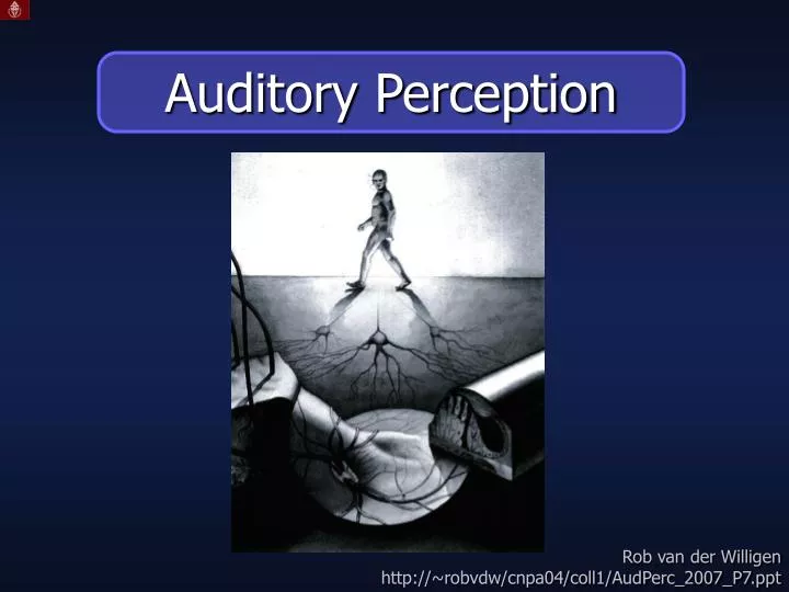
Auditory Perception. Rob van der Willigen http://~robvdw/cnpa04/coll1/AudPerc_2007_P7.ppt. Today’s goal. Understanding masking: Critical bands in masking Power spectrum model of masking Measurement of masking. Psychoacoustics. SPL is not a measure of Perceived Loudness.

E N D
Auditory Perception Rob van der Willigen http://~robvdw/cnpa04/coll1/AudPerc_2007_P7.ppt
Today’s goal Understanding masking: Critical bands in masking Power spectrum model of masking Measurement of masking
Psychoacoustics SPL is not a measure of Perceived Loudness • Defined as the attribute of auditory sensation in terms of which sounds can be ordered on a scale extending from quiet to loud. • Two sounds with the same sound pressure level may not have the same (perceived)loudness • A difference of 6 dB between two sounds does not equal a 2x increase in loudness • Loudness of a broad-band sound is usually greater than that of a narrow-band sound with the same (physical) power (energy content) Recapitulation last weeks’ lecture
Psychoacoustics Perceived Loudness: phone • A unit of LOUDNESS LEVEL (L) of a given sound or noise. • Derived from indirect loudness measurements • If SPL at reference frequency of 1kHz is X dB • the corresponding equal loudness contour is the X phon line. • Phon units can’t be added, subtracted, • divided or multiplied. • 60 phons is not 3 times louder than 20 phons! • The sensitivity to different frequencies is more • pronounced at lower sound levels than at higher. • For example: a 50 Hz tone must be 15 dB higher • than a 1 kHz tone at a level of 70 dB Recapitulation last weeks’ lecture
Psychoacoustics Loudness Scaling: Magnitude of perceptual change Fechner predicted that a JND for a faint background produces the same difference in sensation as does the JND for a loud stimulus. Thus, a scale of S (Loudness) should be derivable by counting intensity jnds Measure of loudness: sensation intensity (S) in JND units Recapitulation last weeks’ lecture
Psychoacoustics Loudness Scaling: Magnitude of perceptual change • Consequences of a logarithmic Loudness function: • Changes from 15 to 30 dB should be the same as the change from 30 to 60 dB. • If loudness additivity holds, two tones at 70 dB should sound as loud as one tone at 140 dB • What if the jnd does not represent a constant change in loudness? • How could this be? • The jnd is determined by two things: • 1) Perceptual distance (change in loudness) • 2) Internal noise Fechner assumed (incorrectly) that internal noise is constant. Measure of loudness: sensation intensity (S) in JND units Recapitulation last weeks’ lecture
Psychoacoustics Loudness Scaling: Stevens’ Power law Another function relating Loudness S is Stevens’ power law: The exponent m describes whether sensation is an expansive or compressive function of stimulus intensity. The coefficient a simply adjusts for the size of the unit of measurement for stimulus intensity threshold above the 1-unit stimulus. =0.3 Recapitulation last weeks’ lecture
Psychoacoustics Scaling: Stevens’ Power law
Psychoacoustics Loudness Scaling: sone vs. phon SONE: a unit to describe the comparative loudness between two or more sounds. One SONE has been fixed at 40 phons at any frequency (40 phon curve). 2 sones describes sound two times LOUDER than 1 sone sound. A difference of 10 phons is sufficient to produce the impression of doubling loudness, so 2 sones are 50 phons. 4 sones are twice as loud again, viz. 60 phons. p is the base pressure of a sinusoidal stimulus, po is its absolute threshold.
Psychoacoustics Loudness Scaling Depends on: Number of excited hair cells (hence bandwidth of sound) Excitation of each cell (energy in each auditory filter)
Psychoacoustics Measuring Sound: Frequency Domain
The Intensity Density Level of three types of NOISES: Psychoacoustics Physical parameters of sound waves: Power Spectrum Density WHITHE NOISE BROWN (RED) NOISE GRAY NOISE Intensity density level [dB] Log Frequency [Hz]
Low Pass High Pass Frequency Frequency Band Pass Band Reject Frequency Frequency Psychoacoustics Measuring Sound: Filter Characteristics
Acoustic Filtering of the Auditory system: A-weighting The shapes of equal-loudness contours have been used to design sound level meters (audiometer). At low sound levels, low-frequency components contribute little to the total loudness of a complex sound. Thus an A weighting is used to reduces the contribution of low- frequencies.
Acoustic Filtering of the Auditory system: Audiograms of non-humans also shows weighting
Psychoacoustics Measuring Sound: Filter boundaries
Psychoacoustics What is Masking? • “The process by which the threshold of audibility for one sound is raised by the presence of another (masking) sound.” • (American Standards Association, 1960) • How can masking occur? • 1) Excitation: Swamping of neural activity due to masker. • 2) Suppression: Reduction of response to target due to presence of masker.
Psychoacoustics What is Masking? Simultaneous / Time Shifted The presence of one sound masks (hides) the presence of another A loud sound will mask a quieter sound (even if presented before (forward masking) or after (backward masking) the quieter sound) e.g. Given a masking tone of 400 Hz 70dB of SIL, a 600 Hz has to be >100 dB SIL than its minimal threshold level (i.e., threshold in quiet) in order to become audible in presence of the 400 Hz masker tone.
Psychoacoustics Temporal aspects of Masking (1) Post-stimulus/Forward/Post-masking: 1st Masker 2nd test tone (2) Pre-Stimulus/Backward/Pre-masking: 1st test tone 2nd Masker (3) Simultaneous Masking: Test tone and Masker together
Psychoacoustics Two Definitions of Masking The process by which the threshold of audibility for one sound is raised by the presence of another (masking) sound. The amount by which the threshold is raised by the masker (in dB).
Psychoacoustics Critical bands in Masking Fletcher (1940) conducted an simultaneous masking experiment in which there was band-pass noise and a single sine wave. The frequency of the sine wave was always at the center frequency of the noise, and the power density of the noise was fixed. The bandwidth of the noise was varied, and for each bandwidth the minimum intensity at which the sine wave could be perceived was determined. With increasing bandwidth, the total energy of the noise increased.
Psychoacoustics Critical bands in Masking Handbook of Psychology By Irving B. Weiner, Donald K. Freedheim, John A. Schinka, Wayne F. Velicer, Alan M. Goldstein http://books.google.com/books?id=fErelr18MEUC&pg=PA87&lpg=PA87&dq=%22Fletcher+(1940)+%22++masking+experiment&source=web&ots=vz3C3Mzhgb&sig=EgANuNFgxcVLWlmnj9oWQYIDD9I#PPA88,M1
Psychoacoustics Critical bands in Masking
Psychoacoustics Critical bands in Masking A sine (signal) in the presence of noise that has a band width (in frequency) centered around the signal. critical band The wider the noise bandwidth the more the signal (sine wave) is masked. Past a particular (frequency) band-width beyond which the threshold doesn’t increase.
Critical band 150 Hz 300 Hz 400 Hz Auditory filter bandwidth 450 Hz 600 Hz Physical bandwidth SPL (dB) Frequency(Hz) 2000 Hz Psychoacoustics Critical band: ERB The transition point of the auditory filter is known as the Critical Band. This has also been termed the Equivalent Rectangular Bandwidth (ERB). • The critical band is the • point at which thresholds • no longer increase. • Conceptually very • powerful, but not much • use in providing an • accurate estimate of filter bandwidth. • Not possible to discern • filter shape from results.
Critical band = ERB 400 Hz Auditory filter bandwidth SPL (dB) Frequency(Hz) 2000 Hz Psychoacoustics Critical band versus Critical Ratio
Psychoacoustics Masking Curves versus ISO-L curves (left Column) Probe threshold, Lp, or Masker threshold, Lm, plotted with fp, as independent variable, will be referred to as "masking curves." (right column) Curves for a fixed probe frequency and with fm as the independent variable will be referred to as "iso-Lp curves" when the masker level Lm, (at probe threshold) is plotted as a function of fm. For plots of the probe level Lp as a function of the masker frequency we will use the term "iso-Lm curves."
Psychoacoustics MASKING CURVE Experimental procedure: The procedure for a masking experiment. (a) The threshold is determined across a range of frequencies. Each arrow indicates a frequency where the threshold is measured. (b) The threshold is re-determined at each frequency (small arrows) in the presence of a masking stimulus (large arrow)
Psychoacoustics The Masking Curve Shown is the hearing curve (red) and a single tone (sine-wave) with a frequency of 1kHz (black). The green curve is the masking curve due to that tone.Indicates the amount that the threshold is raised in the presence of a masking noise centered The band of noise in yellow at a centre frequency of about 1.5kHz cannot be perceived by the human ear because of the masking effect of the tone at 1kHz.
Psychoacoustics ISO-Lp curves (Lm versus Fm): Psychophysical Tuning Curve Experimental procedure: First, a low level test tone is presented. Then, masking tones are presented with frequencies above and below the test tone. Measures are taken to determine the level of each masking tone needed to eliminate the perception of the test tone. Assumption is that the masking tones must be causing activity at same location as test tone.
Psychoacoustics ISO-Lp curves (Lm versus Fm): Psychophysical Tuning Curve The psychophysical tuning curve is determined by measuring the sound pressure of each masking tone that reduces the perception of the test tone to threshold. The procedure for measuring a psychophysical tuning curve. (a) A 10-dB SPL test tone (blue arrow) is presented. (b) Then a series of masking tones (red arrows) are presented at each frequency.
Psychoacoustics Psychophysical tuning curves: ISO-Lp curves (Lm versus Fm) Psychophysical Tuning Curves (PTCs): Fixed signal; masker level adjusted to just mask signal. Psychophysical tuning curves for a number of test-tone frequencies (dots). Notice how the minimum masking intensities for the curves match the shape of the audibility curve (dashed line). (Based on Vogten, 1974). Advantages: Concept v. similar to neural tuning curves, allowing direct comparisons. Potential problems: “Off-frequency listening” Detection of beats if using a sinusoidal masker.
Psychoacoustics Psychophysical tuning curves: ISO-Lp curves (Lm versus Fm) (a) Three human psychophysical tuning curves generated using the method described in right figure. The arrows show the frequency of three different test tones. You can see from the figure that when the masking tone is the same as, or close to, the test tone in frequency, the intensity of the masker needed to mask the test tone is low. (b) Three neural tuning curves showing the stimulus intensity needed to generate a constant response (firing rate) in the nerve fiber of a cat. Each curve represents a different auditory nerve fiber The procedure for measuring a psychophysical tuning curve. A10 dB test tone (black arrow) is presented and then a series of masking tones (red arrows) are presented at the same time as the test tone. The psychophysical tuning curve is generated by determining the SPL threshold of the masking tones needed to reduce the perception of the test tone to threshold Vibration patterns on the basilar membrane caused by 400, 800 and 1000 Hz tones
Psychoacoustics Psychophysical tuning curves versus Frequency Tuning Curves Frequency Tuning Curves (FTCs): measured by finding the pure tone amplitude that produces a criterion response in an 8th nerve fiber. Psychophysical Tuning Curves (PTCs): Fixed signal; masker level adjusted to just mask signal.
Psychoacoustics Summary ISO-Lp curves (Lm versus Fm) or PTC Resulting tuning curves show that the test tone is affected by a narrow range of masking tones. Psychophysical tuning curves (PTC) show the same pattern as neural tuning curves which reveals a close connection between perception and the firing of auditory fibers Advantages: Concept v. similar to neural frequency tuning curves (FTC), allowing direct comparisons. Potential problems: “Off-frequency listening” Detection of beats if using a sinusoidal masker.
Psychoacoustics TWO_TONE SUPRESSION In single auditory nerve recordings, the response to a just supra threshold tone at CF can be reduced by a second tone, even though the tone would - itself have increased the nerve's firing rate. A similar effect is found in forward masking. The forward masking of tone a on tone c can be reduced if a is accompanied by a third tone b with a different frequency, even though b has no effect on c on its own.
Psychoacoustics Iso-Lm curve (Lp versus Fp): Masked Audiogram Lp as function of Fp Masking curves (masked audiograms) for a narrow band of noise centered at 1 kHz and bandwidth of 160 Hz. (Lm is constant) Each curve shows the elevation in the threshold of sinusoidal signal as a function of signal frequency. That is: for a fixed narrowband masker, the change in threshold for a single-tone probe over a specific frequency range is determined. The overall noise level of each curve is indicated in the figure.
Psychoacoustics Shape of auditory filter: Excitation patterns The shape of auditory filters as determined from the shape of tuning curves in masking experiments
Psychoacoustics Shape of auditory filter: Power Spectrum Model The auditory filters can be approximated by rectangular filters, but better determination of the filter shape is possible. The critical bandwidth at a particular frequency can be estimated using the formula where P is the intensity of the signal, N0 is the noise power over a 1-Hz range, K is the threshold of detectability (usually 0.4), and W is the critical band width (CB). N0 is independent of frequency. For example, the CB at 1000 Hz is 160 Hz; however, in reality rectangular filters are not accurate; the shape changes with frequency and amplitude Better approximations of the auditory filters look like this: 160 Hz Auditory filter bandwidth Critical band SPL (dB) Frequency(Hz) 1000 Hz
Psychoacoustics Power Spectrum model of Masking • Fletcher's experiment led to a model of masking known as the power-spectrum model that is based on the following assumptions: • 1. The peripheral auditory system contains an array of linear overlapping band-pass filters. • The non-linearity of the filters is now well known. • 2. Listener detect signals by using just one filter with a center frequency close to that of the signal. • Listeners clearly combine information across filters • 3. Only the components of the noise which pass through the filter have any effect in masking the signal. • Energy outside the filter can play an important role (see literature on informational masking and co-modulation masking release) • 4. Detection threshold is determined by the amount of noise passing through the filter, calculated as the ratio of the long-term power spectra of signal and noise. • Fluctuations in the masker can play a strong role
Hypothetical auditory filter masker masker signal Psychoacoustics Shape of auditory filter: notched noise method
Psychoacoustics Shape of auditory filter: notched noise method The deviation from each of the noise edges to the signal frequency is denoted by delta f. The measurement consists of determining the signal threshold for different notch widths, while maintaining the level of the noise masker constant. Since the signal is symmetrically placed at the center of the notch, the method cannot reveal any filter asymmetries. As the width of the notch is increased, less and less noise leaks through the filter skirts and the threshold is reduced. The variation in threshold with notch width can be seen as a measure of the area of the noise leaking through the filter skirts. Then, assuming that threshold corresponds to a constant signal to masker ratio, the filter function can be obtained by differentiating the threshold function respect to delta f, given that the integral of a function between certain limits corresponds to the area under that function. This is the basic idea that has been used to determine the filter shapes using this method.
Psychoacoustics Shape of auditory filter: notched noise method The "notch-noise method" involves the determination of the detection threshold for a sinusoid, centered in a spectral notch of a noise, as a function of the width of the notch. On the basis of results obtained with this method, auditory frequency selectivity can be described in terms of an "equivalent rectangular bandwidth" (ERB) as a function of center frequency. Both spectral and temporal analysis contribute to the detection of the sinusoid. The CB and the ERB have been found to be proportional for center-frequencies above 500 Hz. • Advantages: • No influence of beats. • Allows accurate measurement of filter “tails” (remote regions). • Analysis can take into account off-frequency listening.
Psychoacoustics Shape of auditory filter: notched noise method The shape of the auditory filter centered at 1 kHz, plotted for relative response of the filter in dB as a function of fequency.
Adjustable signal Fixed masker ‘upward spread of masking’ Psychoacoustics Iso-Lm curve (Lp versus Fm) or Masked Audiograms High-intensity maskers spread their effect towards high frequencies. A response of the Basilar Membrane.
Psychoacoustics Iso-Lm curve (Lp versus Fm): Beating TONE-TONE masking causes BEATS: The masking patterns from masked audiograms do not reflect the use of a single auditory filter. Rather, for each signal frequency the listener uses a filter centered close to the signal frequency. Thus the auditory filter is shifted as the signal frequency is altered. Moreover, varying the frequency distance between two tones results in changed perception. A sense of roughness emerges for distances below a certain threshold (Rocchesso). If the frequencies are far enough apart we perceive two tones. As they close a sensation of roughness emerges, but the separate tones can still resolved. As they get even closer, we stop perceiving two separate tones and hear a single tone that beats.
Psychoacoustics Excitation patterns or Masked Audiograms Moore and Glasberg(1983) presented a simple method for obtaining an estimate of the “internal representation”of any arbitrary signal. To be precise, it is the output of the bank of auditory filters calculated by the Patterson(1976) method. As a simplification, the tails of the filter are ignored, removing the parameter from the equation, leaving the following This allows the output of a bank of filters to be easily calculated for any input.
Psychoacoustics Excitation patterns or Masked Audiograms Given auditory filter shapes, it is possible to derive masking patterns for any arbitrary stimulus. Under the power spectrum model assumptions, a masking pattern is equivalent to an excitation pattern – the internal representation of a sound’s spectrum. • But does masking pattern = excitation pattern?
Psychoacoustics Excitation patterns or Masked Audiograms The shapes of excitation patterns for narrowband stimuli as a function of level can be determined approximately from their masking patterns. The patterns closely resemble masked audiograms at similar masker levels, showing the classic "upward spread of masking." Moore and Glasberg (1987b) concluded that the critical variable determining the auditory filter shape is the input level to the filter.
Cochlear nonlinearity Active processing of sound CF= 9 kHz Response in dB OUTPUT Response in dB ~4.5kHz INPUT level (dB SPL) Frequency [kHz] The response of the BM at location most sensitive for ~ 9 KHz tone (CF). The level of the tone varied from 3 to 80 dB SPL (iso-intensity contours). BM input-output function for a tone at CF (~9 kHz, solid line) and a tone one octave below (~4.5 kHz) taken from the iso-intensity contour plot.