Download
1 / 12
120 likes | 202 Views
Analyzing time-course data with two conditions to assess dampening effect using permutation testing. Measures average change over time points to compare conditions. Interpretation and significance of results explained.

E N D
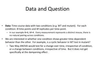
Data and Question • Data: Time course data with two conditions (e.g. WT and mutant). For each condition: N time points and M replicates per time-point. • In our example N=6, M=4. Every measurement represents a distinct mouse, there is no natural pairing across conditions. • We are interested in whether one condition shows greater time-dependent behavior than the other. For example, is a cyclic behavior in WT lost in mutant? • Two-Way ANOVA would test for a change over time, irrespective of condition, or a change between conditions, irrespective of time. But it does not get specifically at the dampening effect .
Un-Paired Series Interrogator for a Dampening Effect (UPSIDE) • The null hypothesis: Each measurement has the same distribution in both conditions. • The null hypothesis must be general, due to the nature of permutation testing. The dampening effect itself is captured in the choice of test statistic , as defined below. • Test Statistic: For a set of data, let the“average change” be the average over all time points of Δs / Δt, where Δs is the change in (average) signal from time point t to t+1, andΔt is the length of the time interval from time t to time t+1 • This statistic is sensitive to non-uniform behavior over time and should be relatively blind to any other effects. • We test the null hypothesis with a one-sided test of the Average Change statistic, using a permutation (aka resampling) test. Under the null hypothesis, the distributions of values from both conditions are the same. • The permutations are derived from resampling M replicates per time point from the pool of all measurements from both conditions, for that time point. • Before resampling, the data are mean normalized (independently in each condition) so that the average time course in each condition is balanced around zero. This normalization assures that any observed difference are due only to a change in shape and not in overall level of intensity.
Interpretation • Under the null hypothesis, the average difference of the original data should not be extreme with respect to this distribution. • Therefore, the tail probability of the observed value of the statistic on the unpermuted data gives a p-value for rejecting the null hypothesis. A small p-values indicates a difference in the data generating WT and mutant. • Since the statistic is designed to be sensitive to the average change, a small one-sided p-value indicates the difference is due to a dampening of the non-uniform behavior over time in the mutant as compared to the WT.
Example: Per3WAT Cre GAPDH KD No-Cre = control No-CreAve Change = 1.246863415
The orange shaded values are a random sample, four values for each time point. Red line = resampled data Ave Change = 0.696599 Blue line = original data no-cre control Red line = original data crekd
Plot of the Ave Change of the Original No-Cre data. • The original value should not be an extreme value if the null hypothesis is true.
P-Value of No-Cre Ave Change Shaded area, the probability of the No-Cre Ave Change or more extreme, gives a p-value for rejecting the null hypothesis. P-value = 0.0085. So only 85 of the 10,000 permutations resulted in an Ave Change value equal or greater than the observed No-Cre control.
Significant P-Values and Multiple Testing • GAPDH_WAT_Bmal1: 0.001 • GAPDH_WAT_Npas2: 0.1497 • GAPDH_Cry1: 0.5819 • GAPDH_Cry2: 0.5837 • GAPDH_Per1: 0.314 • GAPDH_Per2: 0.2529 • GAPDH_WAT_Per3: 0.0085 • GAPDH_Dbp: 0.0689 • GAPDH_e4bp4: 0.0843 • no fast APDH_Reverba: 0.0004 • GAPDH_Reverba: 0.0013 • GAPDH_Cry1: 0.6341 • GAPDH_Cry2: 0.6497 • GAPDH_Per1: 0.3161 • GAPDH_Per2: 0.255 • GAPDH_Dbp: 0.0607 • GAPDH_e4bp4: 0.0545 • BAT_Bmal1 1343 no fast: 0.005 • BAT_Reverba_GAPDH no fast: 0.0551 • BAT_Npas2_GAPDH no fast: 0.9993 • BAT_Cry1_GAPDH no fast: 0.9149 • BAT_Cry2_GAPDH no fast: 0.4221 • BAT_Per1_GAPDH no fast: 0.0894 • BAT_Per2_GAPDH no fast: 0.0523 • BAT_Per3_GAPDH no fast: 0.0477 • BAT_Dbp_GAPDH no fast: 0.0011 • BAT_e4bp4_GAPDH no fast: 0.7431 • BAT_Bmal1 1342 fast: 0.0001 • BAT_Reverba_GAPDH fast: 0.0043 • BAT_Npas2_GAPDH fast: 0.7456 • BAT_Cry1_GAPDH fast: 0.4778 • BAT_Cry2_GAPDH fast: 0.0572 • BAT_Per1_GAPDH fast: 0.0084 • BAT_Per2_GAPDH fast: 0.0207 • BAT_Per3_GAPDH fast: 0.0013 • BAT_Dbp_GAPDH fast: 0.0002 • BAT_e4bp4_GAPDH fast: 0.0096 • 1GAPDH_WAT_Bmal1: 0.013 • GAPDH_WAT_Per3: 0.0288 • GAPDH_WAT_Npas2: 0.8972 Out of 40 tests at the 0.05 level we expect two false positives. We observe 20 significant p-values. We expect therefore that at least 90% of the significant p-values indicate true effects.
Distribution of P-Values • If there are multiple series with no overall dampening effect among them, then the p-values should be uniformly distributed from zero to one. • A skew to the left indicates some of the series present a dampening effect. The more skewed, the more series show the effect. • This example shows the p-values for 40 series. • It is apparent that this is mixture of a uniform distribution (from the genes that are not dampened) and a highly skewed distribution (from the genes that are dampened).


![Cisco 300-170 Dumps Question - Data Networking [300-170] Exam Question](https://cdn4.slideserve.com/7938328/questions-answers-pdf-dt.jpg)