Download
1 / 40
400 likes | 409 Views
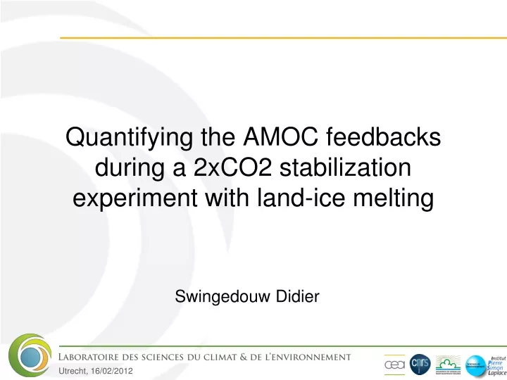
Quantifying the AMOC feedbacks during a 2xCO2 stabilization experiment with land-ice melting. Swingedouw Didier. AMOC spread in projections. Large spread of AMOC response to GHG emissions Gregory et al. 2005: heat flux and freshwater flux both play a role

E N D
Quantifying the AMOC feedbacks during a 2xCO2 stabilization experiment with land-ice melting Swingedouw Didier
AMOC spread in projections • Large spread of AMOC response to GHG emissions • Gregory et al. 2005: heat flux and freshwater flux bothplay a role • Need for understanding processes • Even for a given forcing: large spread Schneider et al., 2007 Stouffer et al. 2006
AMOC and salinity forcing Runoff Precipitations Humidity transport Opposing effects for the water coming from the Arctic and the tropics Salinity advection Evaporation Swingedouw et al. 2007a
Actuel AMOC and salinity forcing Runoff Precipitations Humidity transport Opposing effects for the water coming from the Arctic and the tropics Salinity advection Evaporation Swingedouw et al. 2007a
Actuel Futur AMOC and salinity forcing Runoff Precipitations Humidity transport Opposing effects for the water coming from the Arctic and the tropics Salinity advection Evaporation Swingedouw et al. 2007a
Actuel Futur Futur AMOC and salinity forcing Runoff Precipitations Humidity transport Opposing effects for the water coming from the Arctic and the tropics Salinity advection Evaporation Swingedouw et al. 2007a
Actuel Futur Futur Futur AMOC and salinity forcing Runoff Precipitations Humidity transport Opposing effects for the water coming from the Arctic and the tropics Salinity advection Evaporation Swingedouw et al. 2007a
Actuel Futur Futur Futur Futur AMOC and salinity forcing Runoff Precipitations Humidity transport Opposing effects for the water coming from the Arctic and the tropics Salinityadvectin Evaporation Swingedouw et al. 2007a
Actuel Futur Futur Futur Futur Futur AMOC and salinity forcing Runoff Precipitations Humidity transport Opposing effects for the water coming from the Arctic and the tropics Salinityadvectin Evaporation Swingedouw et al. 2007a
AMOC internal feedbacks Effect – Effect + Salinity density flux AMOCi FCMs Oceanic meridional advection Temperature density flux Stocker et al., 2001
AMOC internal feedbacks Effect – Effect + Freshwater meridional transport Seaice transport and melting Salinity density flux Meridional atmospheric Temperature gradient AMOCi THCe TCMOs Oceanic meridional advection Oceanic meridional heat transport Seaiceamount Temperature density flux Brine rejection Salinity density flux Ekman divergence Stocker et al., 2001
Questions • How to quantify the mechanismsexplaining the response of the AMOC to GHG increase? • Can an additionalfreshwater input lead to substantial AMOC weakening in projections? • What are the roles of feedbacks and forcing for the response of the AMOC?
CO2 (ppm) With 560 No 280 CTL 0 70 500 Ice Snow Ocean Land Experimental design IPSL-CM4 model: • OPA-ORCA2 (0.5°-2°) • LMDz (2.5° x 3.75°) 2xCO2 scenario lasting for 500 years: • With ice sheet melting • No ice sheet melting Temps (années) Time (years)) Net heat flux (Swingedouw et al. 2007b)
JFM mixed layer depth AMOC and convection sites Climatology: Boyer Montegut et al., 2005 • In CTL simulation: AMOC max. of only 11 Sv (obs. around 18 Sv ) • No convection in the Labrador Sea • Overflow of 5.6 Sv (obs. around 6 Sv) IPSL-CM4: CTL
CO2 (ppm) With 560 No 280 CTL 0 70 500 Global temperature No With CTL Model responses Temps (années) • Greenlandicesheet (GrIS) meltingamounts to 0.13 Sv after 200 years and isthen constant • Equivalent melting of GrIS by more than 50% after 500 years=very agressive melting scenario AMOC index Temps (années) No Time (years)) CTL With
Correlation of 0.98 betweendensity in the black box and the AMOC: t=0 No-CTL With-CTL AMOC and density in the convection sites
Influence of haline and thermal response on the AMOC • Withmelting: Changes in temperature (T) and salinity (S) weakens the density (and AMOC)
Influence of haline and thermal response on the AMOC • Withmelting: Changes in temperature (T) and salinity (S) weakens the density (and AMOC) • No melting: Salinity changes explain the recovery
Density budget in the convection box Surface Transport
Density buget in the convection box after 500 years No-CTL With-CTL AMOC increases AMOC decreases Transport Surface Residual Budget
Density buget in the convection box after 500 years Sans-CTRL Avec-CTRL AMOC increases AMOC decreases Transport Surface Résidu Bilan
Synthesis of important factor explaining density budget in No ice sheet melting • Over 500 years AMOC reductionmainlycaused by: • Warming in the convection sites (26 %) • Salinity transport by the overturning (65 %) • AMOC recoverymainlycaused by: • Transport of salinity anomalies by the gyre (40 %) • Seaicemeltingreduction in the convection sites (28 %)
Seaice transport in CTL Sea ice melting anomalies • CTL: • Seaice transport through Fram Strait • Brine rejection in winterwhenseaiceforms Sv CTL No • No melting projections (after 500 years): • Seaice transport decreases • Brine rejection decreases + =
Salinity anomalies in the Atlantic SSS anomalies: No melting- CTL
Linear feedback model (Hansen et al., 1984, for climate sensitivity): G0: Static gain λi: Feedback factors + - Feedback amplification
Weisolate GrIS meltingeffect: Feedback quantification methology now stands for the differencebetween the projections with
Salinity Density flux AMOC_out AMOC_in Climatic system transfer + - Temperature Density flux Dynamical gain: Quantification of feedback factors +
Salinity density flux Ocean transport AMOCin AMOCout + - Local atmospheric damping Temperature density flux Quantification of feedback factors Transport Surface Résidu Transport Surface Résidu Salinity Temperature Heat flux feedback stronglydampsheat transport feedback
Salinity Density flux AMOC_out AMOC_in Climatic system transfer + - Temperature Density flux Quantifying the AMOC feedbacks among different AOGCMs • For a given freshwater input, large spread among AOGCMs (Stouffer et al. 2006) • Methodology of feedbacks quantification could be useful (Swingedouw et al. 2007) • Application to the models from this project framework? + Stouffer et al. 2006
THOR water hosing • 6 models including one OGCM • 1965-2005 with 0.1 Sv
An hypothesis to explain AMOC spread THOR project: Swingedouw et al., in prep. Rypina et al. 2011
Outlooks • Quantifying AMOC feedbacks in the different EMBRACE models • Evaluatingimpact of gyre asymmetry on gyre feedbacks factor • Limits/challenges • Computation of density budget in a model • Assumptionof AMOC related to density in convection zone holdsin othermodels
Predefined sections across the North Atlantic connection with the Arctic ocean overflows : connection between the subpolar gyre and the Nordic Seas reference salinity : 34.8 interface between the subtropical and subpolar gyres AR7W A25 42N OVIDE 26N RAPID
predefined sections and areas defined by (lat,lon) of end points + additional sections FCVARfrom Julie Deshayes: Diagnostic package of 3D metrics of the circulation identify sections and areas as sequences of grid points load grid points scale factors model configurations and simulations load data u, v, θ, S (t,z,y,x) extract data (t,z,l)along sections and areas GFDL CM3 CNRM CM5 IPSL CM5 CCSM4 + HADGEM2 ? + HADGEM3 ? pre-industrial control runs monthly output + ocean-only simulations ORCA2-OON2 ORCA1-OCEP09 ORCA025.L75-G85 GLORYS2V1 • calculate indices (t) for sections, ie components of the northward transport of mass, heat and salt: • net (with and without net mass flux) • overturning in vertical coordinates • overturning in density coordinates • barotropic • baroclinic (net-overturning-barotropic) • 0 to1000m deep • 1000 to 2000m deep • 2000m deep to bottom • related to thermal wind (only from ρ) • calculate indices (t) for areas, regarding heat and freshwater: • volume changes • advective fluxes at ocean boundaries • eddy fluxes at ocean boundaries • diffusion, ice + atmospheric fluxes Matlab package available to the community
Thank you Didier.Swingedouw@lsce.ipsl.fr
Convection sites density as a driver of AMOC? • Strong assumption from the proposed model • Gregory and Tailleux (2010): buoyancy fluxes over the convection sites as a production of Available potential energy then used for Kinetic energy production
Linear feedback factor and hysteresis • Stommel et al. (1961): non linearity for the response of the AMOC to freshwater input • This would appears in the feedback factor of the overturning terms for salinity and heat transport (dependent in the mean state)
Réchauffement climatique - Transport Eau Douce Méridien Action - Action + + Transport, Fonte Glace Flux Densité Salinité Gradient Température Méridien Atmosphérique THCe TCMOs Advection Méridienne Océanique Transport Chaleur Méridien Océanique Formation Glace Flux Densité Température Rejet de Sel Glace Flux Densité Salinité Divergence Ekman, locale + Réchauffement climatique
Avec fonte :convection disparaît Sans fonte :renforcement de la convection en mer de GIN, diminution en mer d’Irminger CTL Réponses des sites de convection Avec : année 500 Sans :année 500
Fonction de courant latitude-profondeur en Atlantique Profondeur Latitude Représentation de la THC dans le modèle • 2 cellules avec NADW et AABW • Maximum pour la NADW d’environ 11 Sv (Indice THC) • Plus faible que les estimations issues d’observations (14-18 Sv) Sv