Download
1 / 111
1.18k likes | 1.44k Views
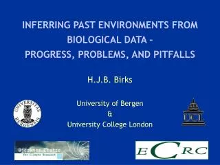
ORDINATION TECHNIQUES IN ENVIRONMENTAL BIOLOGY - PROGRESS, PROBLEMS, AND PITFALLS. H.J.B. Birks University of Bergen and University College London. CONTENTS. INTRODUCTION Definitions Data Types of Ordination Historical Perspective PROGRESS Introduction

E N D
ORDINATION TECHNIQUES IN ENVIRONMENTAL BIOLOGY - PROGRESS, PROBLEMS, AND PITFALLS H.J.B. Birks University of Bergen and University College London
CONTENTS INTRODUCTION Definitions Data Types of Ordination Historical Perspective PROGRESS Introduction Underlying Response Models Indirect Gradient Analysis Direct Gradient Analysis PROBLEMS PITFALLS CONCLUSIONS
INTRODUCTIONDefinitions Ordination - "process of reducing the dimensionality (i.e., the number of variables) of multivariate data by deriving a small number of new variables ('latent variables', 'composite variables', ordination axes) that contain much of the information in the original data. - the reduced data set is often most useful for investigating possible structure in the observations." B.S. Everitt (1998) - "the arrangement of samples or sites along gradients on the basis of their species composition or environmental attributes. Ordination is the mathematical expression of the continuum concept in ecology. Gradient analysis is often treated as a synonym by plant ecologists." M.O. Hill (1998)
End result is a low-dimensional (usually 2 dimensions) plot in which sites are represented by points in two-dimensional space in such a way that points close together in the plot correspond to sites that are similar in species composition, and points that are far apart correspond to sites that are dissimilar in species composition. Plot is a graphical summary of the data. Ordination multidimensional scaling, component analysis, latent-structure analysis Environmental biology - encompasses ecology, environmental monitoring, and palaeoecology. Basically, differences in time scale and temporal resolution only.
Data Data for ordination typically consist of a matrix of values specifying the abundance or presence of species in sites. Environmental data for the same sites sometimes also available. A convenient way to envisage the structure of the data is of two matrices Y and X stacked one beside the other C = [Y|X] = [yij|xik] (i = 1, ......, n; j = 1, ......, m; k = 1, ......, q) Rows of the matrix represent sites. The first block of m columns represents species, yij is the abundance of species j in site i. The second block of q columns represents environmental variables; xik is the value of the kth environmental variable in site i. Given data on species (Y) and environment (X), there are two major approaches to ordination: Indirect gradient analysis - analyse Y only, and then involve X Direct gradient analysis - analyse Y and X simultaneously
Mark Hill Cajo ter Braak Petr Šmilauer
1987 1987 2002 2003
PROGRESSIntroduction Indirect gradient analysis - analyse Y data only Direct gradient analysis - analyse Y and X data together
Aims of Indirect Gradient Analysis • Summarise multivariate data in a convenient low-dimensional way. Dimension-reduction technique. • Uncover the fundamental underlying structure of data. Assume that there is underlying LATENT structure. Occurrences of all species are determined by a few unknown environmental variables, LATENT VARIABLES, according to a simple response model. In ordination trying to recover and identify that underlying structure. • Reasons for using Indirect Gradient Analysis • Species compositions easier to determine than full range of environmental conditions. Many possible environmental variables. Which are important? • Overall composition is often a good reflection of overall environment. • Overall composition often of greater concern than individual species. Global, holistic picture, in contrast to regression which gives a local, individualist reductionist view. • Constrained canonical ordination or direct gradient analysis stands between indirect gradient analysis and regression. Many species, many environmental variables.
Underlying Response Models A straight line displays the linear relation between the abundance value (y) of a species and an environmental variable (x), fitted to artificial data (●). (a = intercept; b = slope or regression coefficient). A Gaussian curve displays a unimodal relation between the abundance value (y) of a species and an environmental variable (x). (u = optimum or mode; t = tolerance; c = maximum = exp(a)).
Indirect gradient analysis can be viewed as being like regression analysis but with the MAJOR difference that in ordination the explanatory variables are not known environmental variables but are theoretical ‘latent’ variables. Constructed so that they ‘best’ explain the species data. As in regression, each species is a response variable but in contrast to regression, consider all response variables simultaneously. ____________________ PRINCIPAL COMPONENTS ANALYSIS PCA CORRESPONDENCE ANALYSIS CA & relative DCA PCA – linear response model CA – unimodal response model
Indirect Gradient Analysis Principal components analysis In regression, fit a particular environmental variable to all the species. Might then repeat for a different environmental variable. For some species, one variable may fit better and for other species, another variable may fit better. Judge the goodness-of-fit (explanatory power) of an environmental variable by the total regression sum-of-squares. What is the best possible fit that is theoretically obtainable within the constraints of the linear response model? Defines the ordination problem - to construct the single hypothetical variable that gives the best fit to the species data according to the linear response model. This hypothetical environmental variable is the LATENT VARIABLE or the first ordination axis.
Principal components analysis provides the solution to this linear ordination problem in any number of dimensions.
PCA results most conveniently presented as BIPLOTS Correlation (=covariance) biplot scaling Species scores sum of squares = λ Site scores scaled to unit sum of squares Emphasis on species Distance biplot scaling Site scores sum of squares = λ Species scores scaled to unit sum of squares Emphasis on sites
Other important questions in PCA • Data transformations. • Data standardisations (covariance or correlation matrix). • Can position 'unknown' samples (e.g., fossil samples) into PCA of 'known' modern samples. • How many axes to retain for interpretation? Comparison with broken-stick model surprisingly reliable. • Interpretation indirect e.g., if environmental data available, overlay or regress variables on PCA axes 1 and 2. If no environmental data, interpret on basis of species biology and ecology.
Correspondence analysis • Invented independently numerous times: • Correspondence Analysis: Weighted Principal Components with Chi-squared metric. • Optimal or Dual Scaling: Find site and species scores so that (i) all species occurring in one site are as similar as possible, but (ii) species at different sites are as different as possible, and (iii) sites are dispersed as widely as possible relative to species scores. • Reciprocal Averaging: species scores are weighted averages of site scores, and simultaneously, site scores are weighted averages of species scores.
Assume we have five species (presences and absences) along a moisture or pH gradient. Can estimate by Gaussian logit regression the moisture optimum of each species. Gaussian logit curve fitted by logit regression of the presences ( at p = 1) and absences ( at p = 0) of a species on acidity (pH). Simple weighted averaging is a good approximation to Gaussian logit regression under a wide range of conditions.
Artificial example of unimodal response curves of five species (A-E) with respect to standardised variables, showing different degrees of separation of the species curves. a: moisture b: First axis of CA c: First axis of CA folded in this middle and the response curves of the species lowered by a factor of about 2. Sites are shown as dots at y = 1 if Species D is present and at y = 0 if Species D is absent.
As a measure of how well moisture explains the species data, can use the dispersion or spread of the species scores or optima. If the dispersion is large, moisture separates the species curves and explains the species data well, under the assumption of a unimodal response model. If the dispersion is small, then moisture is a poor explanatory variable. Is there an environmental variable that would explain the species data better? CA is the technique that will construct the theoretical latent variable that will best explain the species data under the assumption of unimodal species responses i.e., will find the latent variable that will maximise the dispersion of the species scores. The theoretical variable is the first CA axis.
A second CA axis and further CA axes can be constructed so that they also maximise the dispersion of the species scores but subject to the constraint of being uncorrelated with previous CA axes. CA can be applied not only to presence-absence data but also to abundance data. Involves two-way iterative weighted averaging algorithm by starting from arbitary initial values for sites or from arbitary initial (indicator) values for species. Calculate new species scores by weighted averaging of site scores, calculate new site scores by weighted averaging of sample scores, continue until convergence. On convergence, the values are the site and species scores on CA axis 1, and have the maximum dispersion of species scores on CA axis 1. Eigenvalue of axis 1 is the maximised dispersion of the species scores on the CA axis and is a measure of the importance of the ordination axis.
Remarkable feature of correspondence analysis is that it turns out to be the solution to a wide range of seemingly different problems. (Hill, 1974) CA axes can be shown to minimise the ratio of within-species variance of the site scores to the between-species variance, i.e., a CA axis finds the latent variable that separates the species niches or optima as well as possible. Important property of CA in its constrained or canonical form, canonical correspondence analysis. M.O. Hill (1973) J. Ecology 61, 237-249 M.O. Hill (1974) Applied Statistics 23, 340-354
Other important questions in CA • Hill's scaling of scores in multiples of one standard deviation or 'TURNOVER'. Sites differing by 4 SD tend to have no species in common. • Often need to detrend as CA axis 2 may be an artifact, resulting in an arch in CA axis 2. Commonest cause is that there is only one dominant gradient and the second axis may simply be the first axis folded so that axis 2 is a quadratic function of axis 1, axis 3 a cubic function of axis 1, and so on. • Present CA results as biplots with emphasis on species or on sites or symmetric scaling (Gabriel, 2002), or scaled in Hill's turnover standard deviation units, depending on research aims. • Rare species usually have 'extreme' scores - delete them, downweight them, or do not plot them. • Interpretation indirect, as in PCA.
When to use PCA or CA/DCA? PCA – linear response model CA/DCA – unimodal response model How to know which to use? Gradient lengths important. If short, good statistical reasons to use LINEAR methods. If long, linear methods become less effective, UNIMODAL methods become more effective. Range 1.5–3.0 standard deviations both are effective. In practice: Do a DCA first and establish gradient length. If less than 2 SD, responses are monotonic. Use PCA. If more than 2 SD, use CA or DCA. When to use CA or DCA more difficult. Ideally use CA (fewer assumptions) but if arch is present, use DCA.
Hypothetical occurrence of species A-J over an environmental gradient. The length of the gradient is expressed in SD units. Broken lines describe fitted occurrences of species. If sampling takes place over a gradient range 1.5 SD, this means that occurrences of most species are best described by a linear model. If sampling takes place over a gradient range 3 SD, occurrences of most species are best described by a unimodal model.
Methods of indirect gradient analysis or unconstrained ordination of a multivariate set of data, Y
Direct Gradient Analysis Introduction Primary data in gradient analysis Abundances or +/- variables Response variables Y Indirect GA Species Values Predictor or explanatory variables X Direct GA Env. vars Classes
Two-step approach of indirect gradient analysis PCA or CA followed by regression Standard approach from 1954 to about 1985 Limitations: (1) environmental variable studied may turn out to be poorly related to the first few ordination axes. (2) may only be related to 'residual' minor directions of variation in species data. (3) remaining variation can be substantial, especially in large data sets with many zero values. (4) a strong relation of the environmental variables with, say, axis 5 or 6 can easily be overlooked and unnoticed. Limitations overcome by canonical or constrained ordination techniques = multivariate direct gradient analysis.
Direct gradient analysis or canonical ordination techniques Ordination and regression in one technique Search for a weighted sum of environmental variables that fits the species best, i.e. that gives the maximum regression sum of squares Ordination diagram 1) patterns of variation in the species data 2) main relationships between species and each environmental variable Redundancy analysis constrained or canonical PCA Canonical correspondence analysis (CCA) constrained CA (Detrended CCA) constrained DCA Axes constrained to be linear combinations of environmental variables. In effect PCA or CA with one extra step: Do a multiple regression of site scores on the environmental variables and take as new site scores the fitted values of this regression. Multivariate regression of Y on X.
Artificial example of unimodal response curves of five species (A-E) with respect to standardised environmental variables showing different degrees of separation of the species curves moisture linear combination of moisture and phosphate CCA linear combination a: Moisture b: Linear combination of moisture and phosphate, chosen a priori c: Best linear combination of environmental variables, chosen by CCA. Sites are shown as dots, at y = 1 if Species D is present and at y = 0 if Species D is absent.
Combinations of environmental variables e.g. 3 x moisture + 2 x phosphate e.g. all possible linear combinations zj = environmental variable at site j c = weights xj = resulting ‘compound’ environmental variable CCA selects linear combination of environmental variables that maximises dispersion of species scores, i.e. chooses the best weights (ci) of the environmental variables. C.J.F. ter Braak (1986) Ecology 67, 1167-1179
Alternating regression algorithms - DCA - CCA - CA Algorithms for (A) Correspondence Analysis, (B) Detrended Correspondence Analysis, and (C) Canonical Correspondence Analysis, diagrammed as flowcharts. LC scores are the linear combination site scores, and WA scores are the weighted averaging scores.
CCA axis is a linear combination of the environmental variables supplied and it is the 'best' in the sense that it minimises the size of the species niches (minimises the ratio of within-species variance to total variance), and maximises the dispersion of the species scores or optima. Canonical or constrained correspondence analysis • Ordinary correspondence analysis gives: • Site scores which may be regarded as reflecting the underlying gradients. • Species scores which may be regarded as the location of species optima in the space spanned by site scores. • Canonical or constrained correspondence analysis gives in addition: • 3. Environmental scores which define the gradient space. • These optimise the interpretability of the results.
a CCA of the Dune Meadow Data. a: Ordination diagram with environment-al variables represented by arrows. The c scale applies to environmental variables, the u scale to species and sites. the types of management are also shown by closed squares at the centroids of the meadows of the corresponding types of management. b b: Inferred ranking of the species along the variable amount of manure, based on the biplot interpretation of Part a of this figure.
CCA: Biplots and triplots • You may have in a same figure • WA scores of species • WA or LC scores of sites • Biplot arrows or class centroids of environmental variables • In full space, the length of an environmental vector is 1: When projected onto ordination space • Length tells the strength of the variable • Direction shows the gradient • For every arrow, there is an equal arrow to the opposite direction, decreasing direction of the gradient • Project sample points onto a biplot arrow to get the expected value • Class variables coded as dummy variables • Plotted as class centroids • Class centroids are weighted averages • LC score shows the class centroid, WA scores the dispersion of the centroid
Redundancy analysis - constrained or canonical PCA Short (< 2SD) compositional gradients Linear or monotonic responses Reduced-rank regression PCA of y with respect to x Two-block mode C PLS PCA of instrumental variables Rao (1964) PCA - best hypothetical latent variable is the one that gives the smallest total residual sum of squares RDA - selects linear combination of environmental variables that gives smallest total residual sum of squares C.J.F. ter Braak (1994) Ecoscience 1, 127–140 Canonical community ordination Part I: Basic theory and linear methods
RDA ordination diagram of the Dune Meadow Data with environmental variables represented as arrows. The scale of the diagram is: 1 unit in the plot corresponds to 1 unit for the sites, to 0.067 units for the species and to 0.4 units for the environmental variables.
Partial constrained ordinations (partial CCA, RDA, etc) e.g. pollution effects seasonal effects COVARIABLES Eliminate (partial out) effect of covariables. Relate residual variation to pollution variables. Replace environmental variables by their residuals obtained by regressing each pollution variable on the covariables.
Partial CCA Ordination diagram of a partial canonical correspondence analysis of diatom species (A) in dykes with as explanatory variables 24 variables-of-interest (arrows) and 2 covariables (chloride concentration and season). The diagram is symmetrically scaled [23] and shows selected species and standardised variables and, instead of individual dykes, centroids (•) of dyke clusters. The variables-of-interest shown are: BOD = biological oxygen demand, Ca = calcium, Fe = ferrous compounds, N = Kjeldahl-nitrogen, O2 = oxygen, P = ortho-phosphate, Si= silicium-compunds, WIDTH = dyke width, and soil types (CLAY, PEAT). All variables except BOD, WIDTH, CLAY and PEAT were transformed to logarithms because of their skew distribution. The diatoms shown are: Ach hun = Achnanthes hungarica, Ach min = A. minutissima, Aph cas= Amphora castellata Giffen, Aph lyb = A. lybica, Aph ven = A. veneta, Coc pla = Cocconeis placentulata, Eun lun = Eunotia lunaris, Eun pec = E. pectinalis, Gei oli = Gomphoneis olivaceum, Gom par = Gomphonema parvulum, Mel jur = Melosira jürgensii, Nav acc = Navicula accomoda, Nav cus = N. cuspidata, Nav dis = N. diserta, Nav exi = N. exilis, Nav gre = N. gregaria, Nav per = N. permitis, Nav sem = N. seminulum, Nav sub= N. subminuscula,Nit amp = Nitzschia amphibia, Nit bre = N. bremensis v. brunsvigensis, Nit dis = N. dissipata, Nit pal = N. palea, Rho cur = Rhoicosphenia curvata. (Adapted from H. Smit, province of Zuid Holland, in prep) Natural variation due to sampling season and due to gradient from fresh to brackish water partialled out by partial CCA. Variation due to pollution could now be assumed.
Partial ordination analysis (partial PCA, CA, DCA) There can be many causes of variation in ecological data. Not all are of major interest. In partial ordination, can ‘factor out’ influence from causes not of primary interest. Directly analogous to partial correlation or partial regression. Can have partial ordination (indirect gradient analysis) and partial constrained ordination (direct gradient analysis). Variables to be factored out are ‘COVARIABLES’ or ‘COVARIATES’ or ‘CONCOMITANT VARIABLES’. Examples are: 1) Differences between observers. 2) Time of observation. 3) Between-plot variation when interest is temporal trends within repeatedly sampled plots. 4) Uninteresting gradients, e.g. elevation when interest is on grazing effects. 5) Temporal or spatial dependence, e.g. stratigraphical depth, transect position, x and y co-ordinates. Help remove autocorrelation and make objects more independent. 6) Collecting habitat – outflow, shore, lake centre. 7) Everything – partial out effects of all factors to see residual variation in data. Given ecological knowledge of sites and/or species, can try to interpret residual variation. May indicate environmental variables not measured, may be largely random, etc.
Partitioning variance or variation ANOVA total SS = regression SS + residual SS Two-way ANOVA between group (factor 1) +between treatments (factor 2) + interactions + error component Borcard et al. (1992) Ecology 73, 1045–1055 Variance or variation decomposition into 4 components Important to consider groups of environmental variables relevant at same level of ecological relevance (e.g. micro-scale, species-level, assemblage-level, etc.).
a b c d unique unexplained unique covariance Total inertia = total variance 1.164 Sum canonical eigenvalues = 0.663 57% Explained variance 57% Unexplained variance = T – E 43% What of explained variance component? Soil variables (pH, Ca, LOI) Land-use variables (e.g. grazing, mowing) Not independent Do CCA/RDA using 1) Soil variables only canonical eigenvalues 0.521 2) Land-use variables only canonical eigenvalues 0.503 3) Partial analysis Soil Land-use covariables 0.160 4) Partial analysis Land-use Soil covariables 0.142 a) Soil variation independent of land-use (3) 0.160 13.7% b) Land-use structured (covarying) soil variation (1–3) 0.361 31% c) Land-use independent of soil (4) 0.142 12.2% Total explained variance 56.9% d) Unexplained 43.1%
Predictors Covariables Sum of canonical G+C+D - 0.811 D G+C 0.027 G+C - 0.784 G+C D 0.132 D - 0.679 Joint effect DG+C=0.784-0.132=0.679-0.027=0.652 C D+G 0.106 G+D - 0.706 G+D C 0.074 C - 0.737 Joint effect CD+G=0.737-0.106=0.706-0.074=0.631 0.811 0.811 0.812 0.811 Variance partitioning or decomposition with three or more sets of predictor (explanatory) variables Qinghong & Bråkenheim (1995) Water, Air and Soil Pollution 85: 1587–1592 Three sets of predictors – Climate (C), Geography (G) and Deposition of Pollutants (D) Series of RDA and partial RDA
Predictors Covariables Sum of canonical G D+G 0.034 D+C - 0.777 D+C G 0.228 G - 0.538 Joint effect GD+C=0.777-0.228=0.538-0.034=0.549 0.811 0.811 D Covariance terms PD CD CD DG CG CDG DG CDG PC PG CG C G Canonical eigenvalues All predictors 0.811 Pure deposition 0.027 PD Pure climate 0.106 PC Pure geography 0.034 PG Joint G + C 0.132 Joint G + D 0.074 Joint D + C 0.228 Unexplained variance 1 – 0.811 = 0.189
Total explained variance 0.811 consists of: Common climate + deposition 0.095Unique climate PC 0.106 Common deposition + geography 0.013Unique geography PG 0.034 Common climate + geography 0.008Unique deposition PD 0.027 Common climate + geography + 0.544Unexplained variance 0.189 deposition See also Qinghong Liu (1997) Environmetrics 8: 75–85 Anderson & Gribble (1998) Australian J. Ecology 23: 158-167 Total variation: 1) random variation 2) unique variation from a specific predictor variable or set of predictor variables 3) common variation contributed by all predictor variables considered together and in all possible combinations Usually only interpretable with 2 or 3 'subsets' of predictors. In CCA and RDA, the constraints are linear. If levels of the environmental variables are not uncorrelated (orthogonal), may find negative 'components of variation'.