Download
1 / 47
470 likes | 608 Views
CS157A Lecture 13. Revision of Midterm 2. Prof. Sin-Min Lee Department of Computer Science. Relational Calculus. Important features: Declarative formal query languages for relational model Based on the branch mathematical logic known as predicate calculus Two types of RC:

E N D
CS157A Lecture 13 Revision of Midterm 2 Prof. Sin-Min Lee Department of Computer Science
Relational Calculus • Important features: • Declarative formal query languages for relational model • Based on the branch mathematical logic known as predicate calculus • Two types of RC: • 1) tuple relational calculus • 2) domain relational calculus • A single statement can be used to perform a query
Tuple Relational Calculus • based on specifying a number of tuple variables • a tuple variable refers to any tuple
Generic Form • {t | COND (t)} • where • t is a tuple variable and • COND(t) is Boolean expression involving t
Simple example 1 • To find all employees whose salary is greater than $50,000 • {t| EMPLOYEE(t) and t.Salary>5000} • where • EMPLOYEE(t) specifies the range of tuple variable t • The above operation selects all the attributes
Simple example 2 • To find only the names of employees whose salary is greater than $50,000 • {t.FNAME, t.NAME| EMPLOYEE(t) and t.Salary>5000} • The above is equivalent to • SELECT T.FNAME, T.LNAME • FROM EMPLOYEE T • WHERE T.SALARY > 5000
Elements of a tuple calculus • In general, we need to specify the following in a tuple calculus expression: • Range Relation (I.e, R(t)) = FROM • Selected combination= WHERE • Requested attributes= SELECT
More Example:Q0 • Retrieve the birthrate and address of the employee(s) whose name is ‘John B. Smith’ • {t.BDATE, t.ADDRESS| EMPLOYEE(t) AND t.FNAME=‘John’ AND t.MINIT=‘B” AND t.LNAME=‘Smith}
Formal Specification of tuple Relational Calculus • A general format: • {t1.A1, t2.A2,…,tn.An |COND ( t1 ,t2 ,…, tn, tn+1, tn+2,…,tn+m)} • where • t1,…,tn+m are tuple var • Ai : attributeR(ti) • COND (formula) • Where COND corresponds to statement about the world, which can be True or False
Elements of formula • A formula is made of Predicate Calculus atoms: • an atom of the from R(ti) • ti.A op tj.B op{=, <,>,..} • F1 And F2 where F1 and F2 are formulas • F1 OR F2 • Not (F1) • F’=(t) (F) or F’= (t) (F) • Y friends (Y, John) • X likes(X, ICE_CREAM)
Example Queries Using the Existential Quantifier • Retrieve the name and address of all employees who work for the ‘ Research ’ department • {t.FNAME, t.LNAME, t.ADDRESS| EMPLOYEE(t) AND ( d) (DEPARTMENT (d) AND d.DNAME=‘Research’ AND d.DNUMBER=t.DNO)}
More Example • For every project located in ‘Stafford’, retrieve the project number, the controlling department number, and the last name, birthrate, and address of the manger of that department.
Cont. • {p.PNUMBER,p.DNUM,m.LNAME,m.BDATE, m.ADDRESS|PROJECT(p) and EMPLOYEE(M) and P.PLOCATION=‘Stafford’ and ( d) (DEPARTMENT(D) AND P.DNUM=d.DNUMBER and d.MGRSSN=m.SSN))}
Safe Expressions • A safe expression R.C: • An expression that is guaranteed to generate a finite number of rows (tuples) • Example: • {t | not EMPLOYESS(t))} results values not being in its domain (I.e., EMPLOYEE)
Domain Relational Calculus (DRC) • Another type of formal predicate calculus-based language • QBE is based on DRC • The language shares a lot of similarities with the tuple calculus
DRC • The only difference is the type of variables: • variables range over singles values from domains of attributes • An expression of DRC is: • {x1, x2,…,xn|COND(x1,x2,…,xn, xn+2,…,xn+m)} • where x1,x2,…,xn+m are domain var range over attributers • COND is a condition (or formula)
Examples • Retrieve the birthdates and address of the employee whose name is ‘John B. Smith’ • {uv| (q)(r)(s) (EMPLOYEE(qrstuvwxyz) and q=‘John’ and r=‘B’ and s=‘Smith’
Alternative notation • Ssign the constants ‘John’, ‘B’, and ‘Smith’ directly • {uv|EMPLOYEE (‘John’, ’B’, ’Smith’ ,t ,u ,v ,x ,y ,z)}
More example • Retrieve the name and address of all employees who work for the ‘Reseach’ department • {qsv | ( z) EMPLOYEE(qrstuvwxyz) and ( l) ( m) (DEPARTMENT (lmno) and l=‘Research’ and m=z))}
More example • List the names of managers who have at least on e dependent • {sq| ( t) EMPLOYEE(qrstuvwxyz) and (( j)( DEPARTMENT (hijk) and (( l) | (DEPENTENT (lmnop) and t=j and t=l))))}
QBE • Query-By-Example • Supports graphical query language based on DRC • Implemented in commercial db such as Access/Paradox • Query can be specified by filling in templates of relations • Fig 9.5
Summary • It can be shown that any query that can be expressed in the relational algebra, it can also be expressed in domain and tuple relational calculus
Quiz • In what sense doe R.C differ from R.A, and in what sense are they similar?
Relational Algebra • Relational algebra operations operate on relations and produce relations (“closure”) f: Relation -> Relation f: Relation x Relation -> Relation • Six basic operations: • Projection A (R) • Selection (R) • Union R1[ R2 • Difference R1– R2 • Product R1£ R2 • (Rename) A->B (R)
Example Data Instance STUDENT COURSE Takes PROFESSOR Teaches
Natural Join and Intersection Natural join: special case of join where is implicit – attributes with same name must be equal: STUDENT ⋈ Takes ´ STUDENT ⋈STUDENT.sid = Takes.sid Takes Intersection: as with set operations, derivable from difference A B B-A A-B A B
Division • A somewhat messy operation that can be expressed in terms of the operations we have already defined • Used to express queries such as “The fid's of faculty who have taught all subjects” • Paraphrased: “The fid’s of professors for which there does not exist a subject that they haven’t taught”
Division Using Our Existing Operators • All possible teaching assignments: Allpairs: • NotTaught, all (fid,subj) pairs for which professor fidhas not taught subj: • Answer is all faculty not in NotTaught: fid,subj (PROFESSOR £subj(COURSE)) Allpairs - fid,subj(Teaches ⋈ COURSE) fid(PROFESSOR) - fid(NotTaught) ´ fid(PROFESSOR) - fid( fid,subj (PROFESSOR £subj(COURSE)) - fid,subj(Teaches ⋈ COURSE))
Division: R1¸ R2 • Requirement: schema(R1) ¾ schema(R2) • Result schema: schema(R1) – schema(R2) • “Professors who have taught all courses”: • What about “Courses that have been taught by all faculty”? fid (fid,subj(Teaches ⋈ COURSE) ¸subj(COURSE))
Hash STUDENT Merge COURSE Takes by cid by cid The Big Picture: SQL to Algebra toQuery Plan to Web Page Web Server / UI / etc Query Plan – anoperator tree Execution Engine Optimizer Storage Subsystem SELECT * FROM STUDENT, Takes, COURSE WHERE STUDENT.sid = Takes.sID AND Takes.cID = cid
Relational Calculus: A Logical Way ofExpressing Query Operations • First-order logic (FOL) can also be thought of as a query language, and can be used in two ways: • Tuple relational calculus • Domain relational calculus • Difference is the level at which variables are used: for attributes (domains) or for tuples • The calculus is non-procedural (declarative) as compared to the algebra • More like what we’ll see in SQL • More convenient to express certain things
Domain Relational Calculus domain variables Queries have form: {<x1,x2, …, xn>| p} Predicate: boolean expression over x1,x2, …, xn • Precise operations depend on the domain and query language – may include special functions, etc. • Assume the following at minimum: <xi,xj,…> R X op Y X op constconst op X where op is , , , , , xi,xj,… are domain variables predicate
More Complex Predicates Starting with these atomic predicates, build up new predicates by the following rules: • Logical connectives: If p and q are predicates, then so are pq, pq, p, and pq • (x>2) (x<4) • (x>2) (x>0) • Existential quantification: If p is a predicate, then so is x.p • x. (x>2) (x<4) • Universal quantification: If p is a predicate, then so is x.p • x.x>2 • x. y.y>x
Some Examples • Faculty ids • Course names for courses with students expecting a “C” • Courses taken by Jill
Logical Equivalences • There are two logical equivalences that will be heavily used: • pq p q (Whenever p is true, q must also be true.) • x. p(x) x. p(x) (p is true for all x) • The second can be a lot easier to check!
Free and Bound Variables • A variable v is bound in a predicate p when p is of the form v… or v… • A variable occurs free in p if it occurs in a position where it is not bound by an enclosing or • Examples: • x is free in x>2 • xis bound inx.x>y
Can Rename Bound Variables Only • When a variable is bound one can replace it with some other variable without altering the meaning of the expression, providing there are no name clashes • Example: x.x>2 is equivalent to y.y>2 • Otherwise, the variable is defined outside our “scope”…
Safety • Pitfall in what we have done so far – how do we interpret: {<sid,name>| <sid,name> STUDENT} • Set of all binary tuples that are not students: an infinite set (and unsafe query) • A query is safe if no matter how we instantiate the relations, it always produces a finite answer • Domain independent: answer is the same regardless of the domain in which it is evaluated • Unfortunately, both this definition of safety and domain independence are semanticconditions, and are undecidable
Safety and Termination Guarantees • There are syntactic conditions that are used to guarantee “safe” formulas • The definition is complicated, and we won’t discuss it; you can find it in Ullman’s Principles of Database and Knowledge-Base Systems • The formulas that are expressible in real query languages based on relational calculus are all “safe” • Many DB languages include additional features, like recursion, that must be restricted in certain ways to guarantee termination and consistent answers
Mini-Quiz How do you write: • Which students have taken more than one course from the same professor? • What is the highest course number offered?
Translating from RA to DRC • Core of relational algebra: , , , x, - • We need to work our way through the structure of an RA expression, translating each possible form. • Let TR[e] be the translation of RA expression e into DRC. • Relation names: For the RA expression R, the DRC expression is {<x1,x2, …, xn>| <x1,x2, …, xn> R}
Selection: TR[R] • Suppose we have (e’), where e’ is another RA expression that translates as: TR[e’]= {<x1,x2, …, xn>| p} • Then the translation of c(e’) is {<x1,x2, …, xn>| p’}where ’ is obtained from by replacing each attribute with the corresponding variable • Example: TR[#1=#2 #4>2.5R] (if R has arity 4) is {<x1,x2, x3, x4>| < x1,x2, x3, x4> R x1=x2 x4>2.5}
Projection: TR[i1,…,im(e)] • If TR[e]= {<x1,x2, …, xn>| p} then TR[i1,i2,…,im(e)]= {<x i1,x i2, …, x im>| xj1,xj2, …, xjk.p}, where xj1,xj2, …, xjk are variables in x1,x2, …, xn that are not inx i1,x i2, …, x im • Example: With R as before,#1,#3 (R)={<x1,x3>| x2,x4. <x1,x2, x3,x4> R}
Union: TR[R1 R2] • R1 and R2must have the same arity • For e1 e2, where e1, e2 are algebra expressions TR[e1]={<x1,…,xn>|p} and TR[e2]={<y1,…yn>|q} • Relabel the variables in the second: TR[e2]={< x1,…,xn>|q’} • This may involve relabeling bound variables in q to avoid clashes TR[e1e2]={<x1,…,xn>|pq’}. • Example: TR[R1 R2] = {< x1,x2, x3,x4>| <x1,x2, x3,x4>R1 <x1,x2, x3,x4>R2
Other Binary Operators • Difference: The same conditions hold as for union If TR[e1]={<x1,…,xn>|p} and TR[e2]={< x1,…,xn>|q} Then TR[e1- e2]= {<x1,…,xn>|pq} • Product: If TR[e1]={<x1,…,xn>|p} and TR[e2]={< y1,…,ym>|q} Then TR[e1 e2]= {<x1,…,xn, y1,…,ym >| pq} • Example:TR[RS]= {<x1,…,xn, y1,…,ym >| <x1,…,xn> R <y1,…,ym > S }
Summary • Can translate relational algebra into (domain) relational calculus. • Given syntactic restrictions that guarantee safety of DRC query, can translate back to relational algebra • These are the principles behind initial development of relational databases • SQL is close to calculus; query plan is close to algebra • Great example of theory leading to practice!
Limitations of the Relational Algebra / Calculus Can’t do: • Aggregate operations • Recursive queries • Complex (non-tabular) structures • Most of these are expressible in SQL, OQL,