Download

1 / 21
210 likes | 356 Views
Digital Modems. Lecture 1 Fall 2008. Course “mechanics”. Schedule & names for this semester. Every Tuesday, 12 pm-2:15 pm Lecturers Andreas Polydoros Costas Aidinis Stelios Stefanatos {polydoros}, {caidinis}, {sstefanatos}@phys.uoa.gr Offices: Building V, Second floor. Course Outline.

E N D
Digital Modems Lecture 1 Fall 2008
Schedule & names for this semester • Every Tuesday, 12 pm-2:15 pm • Lecturers • Andreas Polydoros • Costas Aidinis • Stelios Stefanatos {polydoros}, {caidinis}, {sstefanatos}@phys.uoa.gr • Offices: Building V, Second floor.
Course Outline • Fundamentals of detection theory • Detection problem formulation • Cost functions • Likelihood ratio • Optimal detection rules (Bayes/Neyman-Pearosn) • Handling of nuisance parameters • Discrete representation of stochastic processes • Signal space/basis • Orthonormal/Karhunen-Loeve expansion • Likelihood functionals • Application in communications • Binary/M-ary systems • Coherent/Non-coherent detection in AWGN • Error probability
Recommended Reading • Course text-book • H. L. Van Trees, Detection, Estimation, and modulation theory • Additional references • J. G. Proakis, Digital Communications • S. M. Kay, Fundamentals of statistical signal processing: Detection theory
Terminology The 'Open Systems Interconnection Basic Reference Model' (OSI Reference Model or OSI Model) is an abstract description for layered communications and computer network protocol design. It was developed as part of the Open Systems Interconnection (OSI) initiative[1]. In its most basic form, it divides network architecture into seven layers which, from top to bottom, are the Application, Presentation, Session, Transport, Network, Data-Link, and Physical Layers. It is therefore often referred to as the OSI Seven Layer Model. The Physical Layer defines the electrical and physical specifications for devices. In particular, it defines the relationship between a device and a physical medium. To understand the function of the Physical Layer in contrast to the functions of the Data Link Layer, think of the Physical Layer as concerned primarily with the interaction of a single device with a medium, where the Data Link Layer is concerned more with the interactions of multiple devices (i.e., at least two) with a shared medium. The Physical Layer will tell one device how to transmit to the medium, and another device how to receive from it (in most cases it does not tell the device how to connect to the medium). Obsolescent Physical Layer standards such as RS-232 do use physical wires to control access to the medium. The major functions and services performed by the Physical Layer are: Establishment and termination of a connection to a communicationsmedium. Participation in the process whereby the communication resources are effectively shared among multiple users. For example, contention resolution and flow control. Modulation, or conversion between the representation of digital data in user equipment and the corresponding signals transmitted over a communications channel. These are signals operating over the physical cabling (such as copper and optical fiber) or over a radio link. Source: http://en.wikipedia.org/wiki/OSI_model
Three-part PHY-layer system model • Tx: Transmitter • Rx: Receiver • Channel: Models the physical distortion • Noise: Thermal noise, interference, …
Block-Diagram Functions of Tx • Source • Discrete or analog • Source coding • Redundancy removal (entropy coding) • Data compression (introducing distortion) • Channel coding • Introduces redundancy to compensate for channel/noise • Data format • Mapping bits to symbols, create packets, frames, e.t.c. • Modulator • Convert the discrete-time input to the continuous-time transmitted waveform Receiver performs the inverse operations
Input Logic Reed-Solomon Convolutional Encoder Puncturing Interleaver Scrambler Data Command Turbo Encoder Puncturing ST Encoder (TSD) Pilot & Data Multiplexer Constellation Encoder Mapping Mapping Pilot Generator IFFT Cyclic Prefix Insertion Output Logic PAPR Scaling IFFT From Rx Adaptivity Control Cyclic Prefix Insertion Output Logic Preambles Generator PAPR Scaling A modern Tx: MIMO/OFDM
Synchronization PAPR Scaling Frame Acquisition Sync Preamble Extraction Cyclic Prefix Extraction FFT Demapper / DC Extraction Input Logic Symbol Offset Estimation Frequency Offset Estimation Joint Symbol Synch Joint Frequency Offset Synch Frame Acquisition Sync Preamble Extraction Demapper / DC Extraction PAPR Scaling Cyclic Prefix Extraction FFT Input Logic Symbol Offset Estimation Frequency Offset Estimation Preambles ST Decoder (TSD) Channel Acquisition Pilots Data Rx Phase Tracking Maximum Ratio Combiner Phase Correction Data Preambles Data Rx Soft Decision Constellation Decoder Convolutional Decoder (Viterbi) De-Interleaver De-Puncturing Reed-Solomon Output Logic Adaptive Metric Calculation LLR Constellation Decoder Turbo Decoder De-Puncturing Noise variance / SNR estimation A modern Rx: MIMO/OFDM
Physical Channel • Distortion-less (LOS) channel: • Two-ray channel: : channel gain : delay
Physical Channel • The two-ray channel is the simplest example of a multipath fading channel • Question: Under what circumstances is the two-ray channel distortion-less • Answer: It depends on the pulse shape • If the channel is (approximately) distortion-less • If the channel inevitably introduces severe distortion
Inference in general • Inference is the task of learning (e.g., making estimations/decisions) based on given data • Examples of inference: • Estimate the path loss introduced by a fading channel • Estimate the range of an enemy aircraft • Predict the stock market’s gain/loss • Decide on which product is best • Decide on which model best fits the observations • In this course we concentrate on a single sub-topic of inference theory: Hypothesis testing (Detection theory) • Emphasis will be given on how the theory is applied to design optimal receiver structures
Decision criteria • A cost function must be defined in order to obtain a detection rule • This function quantifies the cost of taking erroneous decisions • What is the cost of “detecting” an aircraft when it is actually not there? • What is the cost of missing the presence of the aircraft? • After construction of the cost function an optimal decision rule can be obtained that results in minimum cost • The appropriate cost function depends upon the context of the specific problem and is not unique
Hypothesis testing @ Rx side • Problem formulation: • We are given a set of data (observations) • This set could have been generated as the outcome of one of M possible hypothesis • Given the data, and any other statistical information, we want to decide on the correct hypothesis • Examples: • Decide if the data provided by a radar indicate the presence of an aircraft • From a noisy received signal, decide on the transmitted digital sequence
Rx Problem formulation • Radar example: • Binary transmission example: : observed signal : signal generated by the aircraft (if present) : AWGN of power
Rx Problem formulation • In this class, only distortion-less channels will be considered, including AWGN • The observed signals are of the form: • In case the observation is discrete we have : Observation interval where now we use vectors instead of continuous-time functions