Download
1 / 33
350 likes | 451 Views
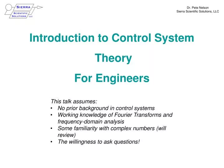
Introduction to Control System Theory For Engineers. This talk assumes: No prior background in control systems Working knowledge of Fourier Transforms and frequency-domain analysis Some familiarity with complex numbers (will review) The willingness to ask questions!.

E N D
Introduction to Control System Theory For Engineers • This talk assumes: • No prior background in control systems • Working knowledge of Fourier Transforms and frequency-domain analysis • Some familiarity with complex numbers (will review) • The willingness to ask questions!
Terminology: dB & the Complex Plane Im i R Lets Practice: 16dB = 6dB + 10dB ~= (2x) x (3x) = 6x 22dB = 10dB + 12dB ~= (3x) x (4x) = 12x 30dB = 10dB + 20dB ~= (3x) x (10x) = 30x 80dB = 4 x 20dB ~= (10x) x (10x) x (10x) x (10x) = 104x 16 bits ~= 16*6dB = 96dB of dynamic range “20dB/Decade” = f(+/-)1 & “40dB/Decade” = f(+/-)2, etc. Some handy Amplituderatios expressed in dB: 0dB = 1x (often used instead of ‘unity gain’ in controls) 6dB ~= 2x [ -6dB ~= 1/2x ] 10dB ~= 3x[ -10dB ~= 1/3x ] 12dB ~= 4x[ -12dB ~= 1/4x ] 20dB = 10x[ -20dB = 1/10x ] Re Euler’s Equation: The Complex Plane: R
Output Input System to control Means to control it What is a Control System? • Example Inputs • and Outputs: • Force • Volts • Heat • Light • Pressure • Example Systems: • House • Hard drive head • Clock osc. • Radio PLL • Power supply • Amplifiers • Example Means: • (sensors & actuators) • Thermistors • Photodiodes • Strain gauge • Disp. Sensor • Heaters • Voice coils But what does this box mean? Input Output
Boxes Represent Transfer Functions: i Im A B( T.F.() B/A ..where B/A is the “Gain” at (phasor diagram) Re • This already means we have made assumptions: • The magnitude of the transfer function (B/A) is constant independent of the magnitude of A. • Linearity and superposition • A single frequency input () produces only a single frequency output without any harmonic distortion, etc. • Linearity again…. • The ratio of B()/A() and the phase () are constant in time. • No saturation! • The input is unaffected by the output and the output is unaffected by load. • ”The signal diode” assumption & ZERO output impedance!
Basic Configuration of a Feedback System: Out In 0 0 G(s) H(s) Transfer function is: Fin -The “Loop Transfer Function” or “Loop Gain” is: Xout M -The “Characteristic Equation” is: H F -Becomes large when: Fin Xout M “G(s)” is the “Plant” transfer function “H(s)” is the “Compensation” Code for “Laplace transform”
+ + X_noise Out In Out H G G Xn H F Xn H H In Out Out G’= In G1 H1 H2 H2 “Block Math”: Multiple Sensors, Nested Loops, & Noise H4 H1 + -The sensor / actuator with the highest gain wins (you can’t have two loops controlling the same DOF at the same time.) H3 F + H5 H2 F
Before we Look Under the Hood… 1) Question: What is on the cover of the Hitchhiker’s Guide to the Galaxy? Don’t Panic The Laplace Transform IS the engine, but you can drive the car without it and you will never need to actually calculate one. 2) The Laplace Transform is used only in continuous-time models; Discretely-sampled (digital) systems require using the Z-Transform. 3) You will get into troubleif you try to use CT techniques in discrete-time (DT) systems. Discrete sampling effects such as aliasing become very significant and compensation filters need special techniques to design. 4) Sorry, but I won’t cover DT and Z-Transforms here. Understanding CT techniques is critical to DT and they will get you “90%” of the way there.
Unstable!!! Im S X 2) The S-plane provides a simple and absolute stability criterion: if any right-half-plane (RHP) poles exist, the system is unstable!!! 0 X Re 0 0 X X 0 X 0 X Think: Why Use the Laplace Transform? Im S 1) The real frequency response is just the Laplace transform evaluated along the positive imaginary axis in the S-plane: L(s) =F(ω) = L(iω) 0 S = iω (S-P1) . Pole-Zero representation: The factorized transfer function takes the form: Re X 0 Then the magnitude of the frequency response is: And the phase angle of the frequency response is:
Xout M Xin 0 0 Mag. (dB) Mag. (dB) Bode Diagram: Bode Diagram: Log(f) Log(f) Phase Phase +180 +180 +90 +90 Log(f) Log(f) 0 0 -90 -90 -180 -180 Figuring Out Transfer Functions Im S Minimal-Phase (θ=90*slope exponent): f 0 X f -2 Re θ = 0 x 90 (plus damping) X θ = -2 x 90 Non-Minimal-Phase (RHP zeros or poles): • Examples: • All-pass filters • Time delays (DT) • “Zero-order hold” (DT) • FIR filters (DT) f 0 Im S Re X 0 Non-minimal phase is always bad in control systems!
If the Characteristic Equation: Has any RHP zeros, the closed-loop transfer function will be unstable. S-plane 1+G(s)H(s) Polar plot of Loop Transfer Function GH: Im Contour enclosing all RHP poles and zeros +∞ freq. Recall: C A B Real frequency response D Gain=1 0 +0 freq. D Re 0 X -0 freq. B 0 Conjugate frequency response A -1 point! C UNSTABLE! -∞ freq. The Nyquist Stability Criterion:
0dB 0dB -0 freq. Mag. (dB) Mag. (dB) Bode Diagram: Bode Diagram: f -1 Log(f) Log(f) Gain=1 f -3 Phase Phase +180 +180 +90 +90 Log(f) Log(f) UNSTABLE! 0 0 -90 -90 +0 freq. -180 -180 A Simple Example….. f -2 Gain=1 f -1 -0 freq. +0 freq. STABLE!
0dB Mag. (dB) Bode Diagram: Log(f) Phase +180 +90 Log(f) 0 -90 -180 Phase is Enemy #1 – Time Delays -0 freq. f -1 Gain=1 phase w/o delay Time delays cause rapidly dropping phase with higher frequency +0 freq. UNSTABLE! Alternate Bode-based stability requirement: The phase must be less than ±180 degrees at unity gain.
Sources of Non-Minimal Phase:The Zero-Order Hold (ZOH) and Transport Delays ADC In DAC out Cts. ∆t t Sampling at 10x unity gain gives ~18 degrees of extra phase! A time delay of 10ms gives ~36 degrees of extra phase at 10Hz! Both effects exist in all digital control systems!
Summary of Section 1: Theory • System Magnitude and Phase responses are represented by complex numbers. In the S-Plane (Laplace Transform Space) by complex poles and zeros. • Pick your Plant (G) to represent the inputs and outputs you care about. The “God Equation” • Systems with Right Half Plane (RHP) poles are unstable. • Introduced a working form of the Nyquist Stability Criterion: || < 180 • → Phase is the enemy. Beware time delays and ZOH! • Introduced Minimal Phase Networks: = n*90, n=power of slope. • Non-minimal phase networks are useless as compensation (exercise for reader). Things we didn’t cover: • Plants with RHP zeros or poles. These are unusual, but can occur, often deliberately! This requires the ‘full version’ of the Nyquist criteria…. (yes, I have lied to you….) • “MIMO” systems: Multiple Input, Multiple Output. This talk only covers “SISO”. • Digital systems require use of the “Z-Transform”. We don’t cover, but its important to learn when you are ready.
0dB Gain Margin Mag. (dB) Bode Diagram: Log(f) Phase Margin Phase +180 +90 Log(f) 0 -90 -180 Dynamic Response: Phase and Gain Margins Gain Margin (STABLE) Gain=1 Phase Margin • Phase Margin usually dominates the closed-loop response • All the information required for dynamic response is in the Bode diagram
A Simple Phase-Margin Calculation: Phasor diagram for 1+GH: 1+GH GH at |GH|=1 Phase Margin θ The vector (1) The Law of Cosines: Gives the amplification: when |GH|=1 (at unity gain) But the real situation is a bit more complex…..
Out In G H Dynamic Response: The Nichols Chart The Nichols chart plots: which is also called the control signal
Bode Diagram: Mag. (dB) Log(f) Phase +180 +90 Log(f) 0 -90 -180 1/f^2 : The Optimal Servo? sensor out + saturation Sensor (or actuator) Saturation: Nom. gain No gain (or negative!) f -3 NEW 0dB sensor in f -<2 Reduced gain 0dB - saturation f -3 UNSTABLE! This is called a “Conditionally Stable” servo Solution: Keep the slope above unity gain to less than 2 powers of frequency.
OK 0dB Mag. (dB) Bode Diagram: Log(f) Phase +180 +90 Log(f) 0 -90 -180 High Bandwidth & Sensor Co-Location: … F H 4 New unity-gain points! ~10x Gain=1 +0 freq. • Eliminate resonances between sensing and actuation • Damp resonances if possible • Increase resonant frequencies (hard!) • Can use filters for isolated resonances 180 degrees for each resonance
Sensors Lie #1: Representation Consider a temperature-control servo: Inner housing Outer housing ~30C outside Insulation Thermistor Heater windings ~60C set pt. Filt & Amp Heater ground Conclusion: Thermal performance is limited by the balancing of heat loss and heat input to ~10% (?!?!). This means servo gains higher than ~20-30dB are a waste!!
0 0 0 Sensors Lie #2: Sensor Noise Xn X2 M2 Xn + Xout M + H F X1 M1 H F Servo wants to minimize the signal here... (Sensor Out) X1 f 0 0 dB f 2 Conclusions: Mass tracks sensor noise Sensor output (noise) suppressed by the loop gain Log(f) Conclusions: Sensor noise is amplified by 1/f2 below the M2resonance!!!!! With ‘1/f’ noise in sensor, mass motion grows by 1,000x each decade (down) to unity gain. Sensor output (noise) suppressed by gain.
Summary of Section 2: Performance • Showed Phase and Gain Margins are useful parameters to describe performance. There is ALWAYS a Phase Margin, but not always a gain margin. • Overshoot (~Q) is ~3x at 20pm, ~2x at 30pm, and critically damped at ~60pm. • Used the Nichols Plot to show that feedback systems rarely look like simple second-order systems. Will demonstrate in Section 3. • Demonstrated there is no ‘right answer’ when it comes to choosing a phase margin. • Proved that a transfer function slope of 1/f2 is the best performing system possible without introducing conditional stability. • Showed mechanical resonances always limit bandwidths and that sensor co-location can mitigate that. • Sensors are lying bastards. If you need to verify performance, use an independent sensor. Things we didn’t cover: • Integrators can reduce errors to zero, and the more integrators the better this works. However ‘integrator wind-up’ is a difficult problem. • The importance of modeling systems. Straight-line approximations only go so far… • PID controllers are horribly non-parametric and only work well for free-mass systems (i.e.: moving stage & motion control). Otherwise they mostly suck. You can do better! • Issues with actually closing the loop on high gain servos – dynamic range and noise!
f -2 phase lead f 0 H Mag. (dB) Mag. (dB) Bode Diagram: Bode Diagram: Log(f) Log(f) Step 2: Design a compensation (H) which pulls the phase down to -180º with enough phase lead at unity gain to give me the desired stability & impulse response. Step 4: Close the loop! Phase Phase +180 +180 +90 +90 Log(f) Log(f) 0 0 -90 -90 -180 -180 How I Design a Servo: Step 1: Model, then measurethe plant transfer function (G): f 0 G f -2 θ = 0 x 90 Step 3: Measure loop transfer function (GH) to confirm. θ = -2 x 90
Compensation Null sensor Damping (phase lead) f -1 H f 1 f -2 0dB 0dB 0dB Filter HF noise 0 Loop Transfer Function Always start with physics: F=ma Mag. (dB) Mag. (dB) Mag. (dB) Bode Diagram: Bode Diagram: Bode Diagram: f -3 GH f -2 Plant f -1 G Log(f) Log(f) Log(f) Units: X/F ! f -2 f -2 f -4 Phase Phase Phase +180 +180 +180 +90 +90 +90 Log(f) Log(f) Log(f) 0 0 0 -90 -90 -90 -180 -180 -180 θ = -2 x 90 = -180 Now With Some More Detail: Remember from start of talk: Xout M H F Fin • Requirements for our servo: • Have a spring-like restoring force • Provide damping • Always bring the sensor to null • Filter noise
+0 freq. 0dB UNSTABLE? CCW encirclement? -0 freq. Im Recall: +0 freq. +∞ freq. S Mag. (dB) Bode Diagram: STABLE Log(f) Real frequency response Gain=1 0 +0 freq. Phase Re 0 X +180 -0 freq. We have THREE poles at the origin! +90 0 Log(f) 0 Conjugate frequency response Contour enclosing all RHP poles and zeros -90 -180 -0 freq. -∞ freq. But is it stable? Loop Transfer Function f -3 GH f -2 f -1 Gain=1 f -2 f -4
Loop T.F.: 0dB 0 G F Recall: Mag. (dB) Mag. (dB) Bode Diagram: Bode Diagram: f 0 f 0 Mag. (dB) Bode Diagram: GH G Log(f) Log(f) f -2 f -2 Log(f) Closed-loop response: ω0 ω0 Phase Phase ω0 +180 +180 Phase θ = 0 x 90 θ = 0 x 90 +90 +90 +180 Log(f) Log(f) 0 0 Original resonance is GONE! +90 Log(f) θ = -2 x 90 θ = -2 x 90 -90 -90 0 -180 -180 -90 -180 The Magic Disappearing Resonance: Consider a mass on a spring: Fin Xout M Plant:
0 0 The “Super Spring” Servo Xout Optical Corner Cube Mref Sensor Meas. Output M 200Hz M Inject Test Signal G F Xin
Summary of Section 3: Practical Design • Start design with a simple, linear, minimal-phase approximation to get 1/f2. • Work backwards from the Plant (G) and the desired LTF (GH) to get H. • Use the alternate version of the Nyquist Stability criteria because polar plots make your head hurt too much. • Closed-loop systems often show no sign of open-loop resonances. • You can add 360 to the phase and get the same plot. Phase works on a circle! High-Freq. resonances can sometimes be tamed by ADDING phase!!! Things we didn’t cover: • Did I already mention modeling? Good. I needed to at least twice! • Sensor noise can also limit bandwidth. In the Super Spring, it grows like 1/f3!! • So many other things. I hope this is just a start!