Download
1 / 54
580 likes | 1.11k Views
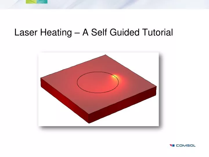
Laser Heating – A Self Guided Tutorial. Introduction. This series of tutorials show how to simulate laser heating of glass. The heating due to laser is treated as a body heat source. The scenarios investigated are: Stationary laser with constant power – CW mode

E N D
Introduction • This series of tutorials show how to simulate laser heating of glass. • The heating due to laser is treated as a body heat source. • The scenarios investigated are: • Stationary laser with constant power – CW mode • Stationary laser with pulsed power – Pulsed mode • Moving laser with constant power – CW mode
Assumptions • Material properties are assumed to be constant. • The electromagnetics of the laser beam is not simulated. • The effect of electromagnetic wavelength is not explicitly modeled. • The effect of complex refractive index of glass is modeled using an absorption and reflection coefficient. • The simulation does not involve modeling phase change.
Model Definition Heat flux = h(Text - T) Glass slab • The modeling geometry only includes the glass slab. • Except the top surface, all other boundaries are assumed to be thermally insulated. • The heat flux on the top surface simulates convective cooling.
Calculating the heat input • The body heat load within the glass slab is given by the following expression. 2D Gaussian distribution in xy-plane Total power input Exponential decay due to absorption Reflection coefficient Reference: "Comparing the use of mid-infrared versus far-infrared lasers for mitigating damage growth on fused silica," Steven T. Yang, Manyalibo J. Matthews, SelimElhadj, Diane Cooke, Gabriel M. Guss, Vaughn G. Draggoo, and Paul J. Wegner. Applied Optics, Vol. 49, No. 14, 10 May 2010.
Information on model implementation • The reflection and absorption coefficients are assumed to be constants. • The planar surface of the glass slab incident to the laser beam is assumed to be aligned with the xy-plane of the global coordinate system. • The top planar surface is aligned with z = 0. Hence the effect of absorption can be simulated by the term exp(-Ac*abs(z)). • The center of the beam can be easily shifted by changing x0 and y0. • The beam width and astigmatism can be easily controlled by the standard deviation parameters; σx and σy.
Case 1: Stationary laser with constant power • This model investigates the transient heating of a glass slab when an incident laser beam in CW mode shines upon it for a given time. Heat flux = h(Text - T) Glass slab
Modeling Instructions • The next few slides show the modeling steps and snapshots of the solution. • For details refer to the model file: laser_heat_transient_CW.mph
Add Physics • Heat Transfer > Heat Transfer in Solids (ht)
Parameters These numerical values are arbitrary and only for illustration purposes
Global Definitions > Functions > Analytic This analytic function represents a 2D Gaussian pulse
The actual geometry This elliptical surface created on the top surface is used to guide a finer mesh in the area where the laser beam is incident upon
Material properties Material Browser > Built-In > Silica glass
Technical note on meshing • We created an extra elliptical boundary on the top surface to represent the zone of heat input. • The shape and position of this ellipse is parameterized. • Use a fine enough mesh only on this ellipse to resolve the Gaussian pulse. • Try to keep the overall mesh count low by using a swept mesh. • * If the absorption coefficient is very large then the heat source would be only effective near the top surface. This would require you to create a graded swept mesh with more layers.
Results – Isosurface Temperature Enable slide show to see the movie
Temperature vs. Time The red dot shows the point of observation
Temperature along top surface The lines on which the solution were plotted are shown in red (x-direction) and blue (y-direction) respectively in the inset picture.
Heat input along top surface Note the x-shift since we had specified x0 = 0.5 mm and y0 = 0 mm
Things to try • Use an Extremely Coarse mesh and solve the model again. How does the solution look? • Go to Global Definitions > Parameters and use a much smaller value of sigx and sigy. Is the same mesh good enough?
Case 2: Stationary laser with pulsed power • This model investigates the transient heating of a glass slab when an incident laser beam in pulsed mode shines upon it for a given time. Heat flux = h(Text - T) Glass slab
Modeling Instructions • The next few slides show the modeling steps and snapshots of the solution. • You can start from the previous model and make changes or add new steps as shown in the following slides. • For details refer to the model file: laser_heat_transient_pulsed.mph
Parameters Note that the value of Q0 is an arbitrary high number that is chosen for illustration purposes only.
Global Definitions > Functions > Analytic This approach can be used to create a series of periodic triangular pulses with variable duty cycle
Variables This is how the effect of pulsed heat input is simulated Multiply the original function with a function of time
Time-Dependent Study • For illustration purposes we have chosen the end_time such that this model will simulate only ten pulses. • Note that solving for a longer time scale will involve more computational time and memory.
Results – Temperature at the center of beam spot as a function of time
Results – Heat input at the center of beam spot as a function of time
Suggestions on time stepping • The choice of intermediate steps provides better resolution of the solution over time without saving the solution at too many small time steps. • This choice could be useful when the input to the model are short pulses. • The default free time stepping may completely ignore these pulses. • The intermediate option involves more computational time than the default free option. • Hence we should always solve the model once with the default free time stepping and inspect the solution to see whether it is lacking any physical behavior.
Solving the same model with free time stepping algorithm • Temperature vs. time behavior does not look correct! • Maximum temperature is underpredicted. • Heat input profile is accurately captured.
Case 3: Moving laser with constant power • This model investigates the transient heating of a glass slab when an incident laser beam in CW mode shines upon it for a given time. • The laser beam also moves over the surface at a given speed along a prescribed path. Heat flux = h(Text - T) Glass slab
Modeling Instructions • The next few slides show the modeling steps and snapshots of the solution. • You can start from the first model and make changes or add new steps as shown in the following slides. • For details refer to the model file: laser_heat_transient_CW_moving.mph
Parameters These numerical values are arbitrary and only for illustration purposes
Variables • Note how the center spot of the beam is obtained from the parametric equation of the path of laser motion. • This is how the time-dependency in the beam position is implemented.
Geometry • We create extra geometric edges on the top surface which outline the path of laser motion. • These edges are used to guide a finer mesh only along the path of laser motion. • Although we use a circular path in this tutorial, in general you could create any arbitrary path using the Parametric Curve or Interpolation Curve geometry features.
Time-Dependent Study • For illustration purposes we have chosen the time_end such that this model will simulate one revolution of the laser beam along the circular path.