Download
1 / 48
480 likes | 650 Views
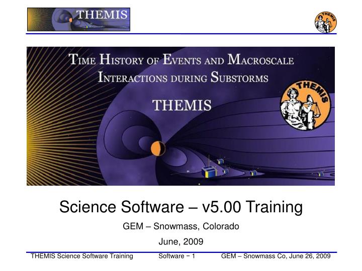
Science Software – v5.00 Training GEM – Snowmass, Colorado June, 2009. Agenda. 10:30 Introduction C. Goethel 10:35 THEMIS Web Site C. Goethel 10:40 V5.00 Science Software/Data Status Report C. Goethel 10:45 THEMIS Science Data Analysis Software C. Goethel

E N D
Science Software – v5.00 Training GEM – Snowmass, Colorado June, 2009
Agenda • 10:30 Introduction C. Goethel • 10:35 THEMIS Web Site C. Goethel • 10:40 V5.00 Science Software/Data Status Report C. Goethel • 10:45 THEMIS Science Data Analysis Software C. Goethel • 11:10 Coordinate Transformation, Plotting, Mapping Tools, Mini-Language P. Cruce • 11:30 V5.00 THEMIS Graphical User Interface (GUI) C. Goethel • 12:15 THEMIS Ground Based Observatories (GBO) P. Cruce • 12:30 SPDF – CDAWeb P. Cruce
Status Report • V5.00 Science Software/Data Status Report • General Loads, introduces and calibrates all L1 quantities, all instruments Loads calibrated L2 quantities • STATE L1 STATE available since launch, V03 STATE (improved attitude and spin phase corrections) - Soon • FGM L1, L2 data available since early March 2007 • FIT / FFT / FBK - L1, L2 data available since early March 2007 • SCM L1 data available since early March 2007 L2 frequency spectrograms (FBK) available now L2 SCM available Summer 2009 • EFI All L1 data available from TH-C since May 2007, TH-D,E since Jun 7 L2 EFI available Fall 2009 • ESA No L1 data, only L0 data – however, read-in is transparent to user All data available since ESA turn-on, i.e., mid-March L2 omnidirectional energy spectrograms, ground moments available now • SST L1 data available since SST turn-on, mid-March L2 omnidirectional energy spectrograms available now • ASI L1 thumbnail images from 21 stations available. L1 full-resolution images available up to November 2008, Mosaics, movies for full mission • GMAG L2 cdf files with ground magnetometer data from 51 stations. That includes one from Greenland and seven from Augsburg College. The Greenland data for the NRSQ station is updated daily and data is provided from October 2008 to present. The other 14 Greenland stations data is provided from 2007 through February 2009. Acknowledgement to Hans Gleisner of the Danish Meteorological Institute for the Greenland data and to Mark Engebretson and Erik Steinmetz for the Augsburg College data. • Other Missions • GOES – The GOES high-resolution (0.5s) magnetometer data is from GOES 10, 11 and 12 satellites from • September 2007–June 2008 for each satellite. Acknowledgement to Howard Singer at • NOAA Space Weather Prediction Center for the data. • ACE - The ACE data consists of magnetometer values in GSM coordinates with one minute averages • and Solar Wind Electron Proton Alpha Monitor data
THEMIS Data Analysis Software Organization Contributors UC Berkeley D Larson, H Frey, J Bonnell, J McFadden, A Keiling J McTiernan, J Lewis UCLA V Angelopoulos, P Cruce, B Kerr, C Goethel, M Feuerstein, K Ramer, H Schwarzl , A Flores SP Systems K Bromund NASA/GSFC V Kondratovich MPE E Georgescu TUBS U Auster CETP P Robert, O LeContel Calgary B Jackel, E Donovan
Overview Overview • Software Objectives • Powerful, Flexible Command Line Interface • GUI to provide Easy Access to Key Features • Software Installation • Data Distribution • Key Routines, crib sheets. • Examples
Software Objectives • Software Objectives • Powerful, Flexible Command Line Interface • GUI provides easy access to data, analysis tools, and graphics • Code is available to everyone, but not required to analyze data. • IDL based (library of routines –but no main program!). • Separates the tasks into: • Reading • Manipulating • Plotting • Platform independent. Works on: • Solaris • Linux • Windows, Vista • Mac OS X
Software Organization - 1 • THEMIS Specific Routines (idl/themis/) • Instrument specific routine organization • Load Data • Calibrate Data • Transforming Data • Crib Sheet Examples .
Software Organization - 2 General routines (idl/ssl_general) Library of generic routines useful for building mission-specific load routines CDF reading/writing routines File retrieval routines Miscellaneous routines Plotting routines Uses “tplot variables”: strings that associate data together with metadata and plotting parameters. Routines to manipulate/plot tplot variables Data Export routines Data Processing routines
Software Organization - 3 External Libraries (idl/external) CDAWlib – from NASA SPDF, reads/plots CDF data IDL_GEOPACK – Magnetic field modelling kit
System Requirements Windows, Solaris, LINUX, PPC Mac or Intel Mac. IDL 6.2 or higher required IDL Patch Recommended Required for Intel Mac, regardless of IDL version Required for IDL 6.2, (Strongly recommended for IDL 6.4 and 7.0) http://cdf.gsfc.nasa.gov/html/cdf_patch_for_idl6x_new.html For Mac, system configurations are required to run IDL Required for Intel Mac, regardless of IDL version X11 – may need to be installed. Mouse click-through one-time X11 configuration necessary for proper operation defaults write com.apple.x11 wm_click_through -bool true See THEMIS User's Guide for full information, available at: ftp://apollo.ssl.berkeley.edu/pub/THEMIS/
Installing/Configuring TDAS Installation Download and expand the latest TDAS release .zip file. The latest version is 5.00. http://themis.ssl.berkeley.edu/socware/tdas_5_00/tdas_5_00.zip Set up the IDL path Windows and IDLDE on any platform: File->Preferences UNIX-like systems (Mac OS X, Linux, Solaris) In .cshrc: setenv IDL_PATH ‘<IDL_DEFAULT>:+/path/to/tdas’ -Or- In .bashrc or .bash_profile: export IDL_PATH=‘<IDL_DEFAULT>:+/path/to/tdas’ Set path to Data Directory Data directory will be created automatically at C:/data/themis (Windows) ~/data/themis (UNIX/LINUX/Max OS X) Run thm_ui_config from command line or THEMIS GUI if you need to change this.
Data Definitions The software operates on Level 1 and Level 2 data. Data Level Definitions: Level 0 Data – Raw files (*.pkt) one per APID. Only used for loading ESA data. Level 1 Data - CDF (Common Data Files) files (*.cdf) Files contain raw, uncalibrated data. i.e. counts, DAC units. Requires TDAS software to interpret. Calibration is done by default when Level 1 data is input. Level 2 Data - CDF files – contain physical quantities – TDAS software is not needed for interpretation. Files available for ESA, FBK, FIT, FGM, MOM*, SST – can be downloaded from SPDF. *(except for MOM)
Data / Directory structure Data Directory structure is large! ~3GB/day for all probes (L1 data) Directory hierarchy keeps directory size manageable Software performs automatic file retrieval. Software maintains directory hierarchy. Behaviour of Automatic File Retrieval is configurable ‘No Download’ mode for stand-alone operation. ‘No Update’ mode to preserve local modifications. Root directory determined automatically, is configurable. Available configuration methods: thm_ui_config IDL widget Button on THEMS GUI widget Environment variables
Primary Routines Load Routine Summary Notes: (*) calibration routine available but still under development - data reduction and analysis routines available: see crib sheet
Primary Routines Usage Conventions: Use keywords to determine functionality level - Calibrated Level 1 data is the default (Except for SST and ESA data, which is handled differently). datatype and probe keywords determine which data is loaded and/or created through calibration process /get_support_data keyword is needed in thm_load_state to load data required by thm_cal* and thm_cotrans routines. To load uncalibrated data, set type = ‘raw’ (For all but SST, ESA) Example from IDL Command Line: timespan,’2007-07-07’,1 ;choose a time range thm_load_state, probe = 'a', /get_support_data thm_load_fgm, probe='a', coord='gsm', datatype='fgl', level=1
Variable Names Probe specification. Example: tha a – can be one of [a-e] specifies probe Particle data. Example: tha_peif p – particles e – ESA, s – SST i – ions, e – electrons f – full, r – reduced, m – moments, b – burst FGM data. Example: tha_fgl l – low telemetry rate, h – high telemetry rate, e – engineering decimated high rate, s – spin fit. Electric Fields and SCM. Example: tha_efs ef - efi, sc – scm, fb – fbk, ff – fft s – spin fit, f – full orbit or fast survey, p – particle burst, w – waves burst. Wildcards are accepted in names when plotting and data processing: th?_fg? th[ab]_fg[lh] th?_state*
Crib Sheets thm_crib_asi thm_crib_dproc thm_crib_efi thm_crib_esa_da thm_crib_esa_moments thm_crib_export thm_crib_fac thm_crib_fbk thm_crib_fft thm_crib_fgm thm_crib_fit thm_crib_gmag thm_crib_mom thm_crib_mva thm_crib_overplot thm_crib_part_getspec thm_crib_scm thm_crib_sst thm_crib_state thm_crib_tplot thm_crib_tplotxy thm_crib_twavpol thm_map_examples Crib Sheets for Loading, Processing and Plotting IDL>.run thm_crib_asi or cut and paste, or copy and modify
Coordinate Transformations Coordinate Transformations thm_cotrans transforms to/from any of the following coordinate systems in a single call updates metadata in output. knows coordinate system of input from metadata Currently Supported Geophysical Coordinate Systems SPG Spinning Probe Geometric SSL Spinning SunSensor L-vectorZ DSL Despun SunSensor L-vectorZ GEI Geocentric Equatorial Inertial GSE Geocentric Solar Ecliptic GSM Geocentric Solar Magnetospheric SM Solar Magnetic GEO Geographic Coordinate System Example (using previously loaded FGM and STATE data) thm_cotrans, 'th?_fg?', out_coord='geo‘, ouf_suffix = ‘geo’
Plotting & Analysis Routines Plotting tplot tplotxy plotxy plotxyz tplot_names tlimit get_data store_data Analytic Coordinate Transformations • tvector_rotate • fac_matrix_make • thm_fac_matrix_make • minvar_matrix_make Tsyganenko Model • (t)trace2iono • (t)trace2equator • (t)t89 • (t)t96 • (t)t01 • (t)t04s Example: tt89,'thc_state_pos',newname='model_field' fac_matrix_make,'model_field' ,other_dim= 'xgse', newname = 'fac_mat' tvector_rotate, 'fac_mat', 'thc_peir_velocity', newname = 'ion_velocity_model_fa'
Command Line Example 1 To load data: timespan,'6-10-2',2,/days thm_load_gmag,site='ccnv',$/subtract_average To plot data: options,'thg_mag_ccnv',$labels=['Bx','By','Bz'] tplot_options, 'title', $'GMAG Examples' tplot,’thg_mag_ccnv’
Command Line Example 2 Wavelet transform on an interval of interest Define and display the interval Tr = ['2006-10-2/16:00','2006-10-3/05'] timebar,tr • Split the 3-vector into components: • split_vec,'thg_mag_ccnv' • Compute transform of one component • wav_data,'thg_mag_ccnv_x',/kol $ ,trange=tr ,maxpoints=24l*3600*2 • Set color limits (log scale) • zlim,'*pow', .0001,.01,1 • Plot it. • tplot,'*ccnv_x*',trange=tr
Plotting Examples tplotxy can be used to plot isotropic position plots. Like plots of magnetic field models and spacecraft position Plotxyz can be used to plot 3 dimensional isotropic data, with any axis.(Not restricted to time-series.)
Plotting Angular Spectra full Pitch angle spectra for full and reduced mode electron ESA data. Plotted using tplot. reduced thm_part_getspec, $ probe=['c'], $ ;select probe trange=['07-06-03/01:08', $ ;select timerange '07-06-03/04:20'], $ data_type=['peef','peer'], $ ;select data type angle='pa', $ ;select pitch angle spectra regrid=[32,16] ;set resolution of pitch/gyrospectra full reduced
Trace / Orbit Plots Trace / Orbit Plots • New routines have been added to perform different 2d projections of 3d data. This particularly useful for plotting orbits and field lines. • A Tsyganenko interface has been added to TDAS that allows us to calculate model field lines for T89,T96,T01,&T04 models. Field lines can also be Traced. • Examples of these routines can be found in themis/examples/thm_crib_trace.pro, themis/examples/thm_crib_plotxy.pro and themis/examples/thm_crib_tplotxy • The graphics in this slide were generated with thm_crib_trace.pro Example: .run thm_crib_trace.pro • A routine was added to plot an arbitrarily sized and spaced AACGM • coordinate grid on a world map. reduced
Trace / Orbit Plots • Trace/Orbit Plots - AACGM/Iono Trace Plot reduced
Trace / Orbit Plots Trace / Orbit Plots – XY Plot reduced
Trace / Orbit Plots Trace / Orbit Plots – XZ Plot reduced
Mini Language THEMIS – Mini Language • Simple scripting language has been written in IDL. • This language allows access to some data analysis functionality in the IDL • virtual machine and eases manipulations of time series data.(tplot) • This language allows composition of statements and functions with order of • operations to give significant flexibility in statement construction. • Examples: • 1: Position to RE: calc,'"tha_pos_re" = "tha_state_pos"/6374.4’ • 2: Natural log of total esa density: • calc,'"tha_density_log" = ln("tha_peir_density"+"tha_peer_density“) • 3: Store tplot data in non-tplot idl variable: calc,'var_data = "tha_efs“’ • 4: Average Magnetic Pressure: • calc,'Pb_avg = mean(0.01*total("tha_fgs_dsl"^2,2)/25.132741)‘ • Additional examples can be found in themis/examples/thm_crib_calc.pro reduced
Trace / Orbit Plots Plotxyvec – Position/Velocity Plot reduced
THEMIS software for GBO all-sky imager Thm_crib_asi.pro Harald U. Frey
All-sky imager data products • Keograms along local magnetic meridian • Delivered daily jpeg-compressed • Reprocessed ½ year later with full resolution images • Geomagnetically mapped thumbnail images • Delivered daily square-root intensity compression • 1024 pixels within +-8o magnetic Latitude and ~+-12o Longitude • 3 seconds temporal resolution • Full resolution images • 256x256 pixels covering about 600 km radius around station • Delivered about ½ year later • 3 seconds temporal resolution • Full 16 bit intensity scale
Mosaic with S/C footprint From thumbnail images Black line marks footprint of THEMIS-P2 during whole night Asterisk marks location at time of mosaic
Ground magnetometer Examples Thm_crib_gmag.pro
Three station example GMAG Data With Average Subtracted
May 7, 2009: THEMIS FGM dataset files being reprocessed at Berkeley and re-ingested into CDAWeb Sep 2008 - Jun 2009: Magnetometer data added from several additional ground stations for a total of now 44 stations from the GBO (31), GEONS (11), and GIMA (2) networks (most recent NAIN, CDRT and NRSQ). SPDF – What’s new CDF: CDF V3.3.0 is in its final testing phase. It adds file validation and sanity checks while accessing CDF files. This addresses potential security vulnerabilities, e.g. data overflow in applications caused by compromised files. Additional functionality and performance improvements were made in the IDL and MATLAB library support. . CDAWeb THEMIS Data:
Eight new geomagnetic activity index variables added to the OMNI 1min and 5min datasets: AE, AL, AU, SYM/D, SYM/H, ASY/D, ASY/H, PC ; already available in OMNI-1hour: daily Rz and F10.7 , 3-hour Kp and ap, 1-hour Dst, AE, AL, AU, and PC New on CDAWeb - Global images and movies of Total Electron Content (TEC) deduced from Global Positioning Satellites (GPS_TEC2HR_IGS) (1998 through present). Excellent data set for monitoring the global ionospheric response to magnetic storms. SPDF – What’s new CDAWeb THEMIS-related Data: Global GPS-TEC image showing the typical Equatorial Anomaly signature with crests on both sides of the magnetic equator.
Level-2 Data from all 5 Satellites for FGM, ESA, SST, FBK, FFT, & FIT data quantities. Ground Magnetometer Data from 44 stations (31 GBO, 11 GEONS, 2 GIMA) Keograms from 23 All-Sky-Imagers (ASI) going back to 2005. All data updated daily (auto-ingest) from THEMIS data site. GIF-Walk: pre-generated Magnetopause Crossing Survey plots (David Sibeck, NASA GSFC) http://cdaweb.gsfc.nasa.gov/cgibin/gif_walk State files with definitive orbits (bi-weekly updates) in all coordinate systems used in SSC and incl. magnetic traces. Very popular data set. CDAWeb: THEMIS Data Summary
Common Data Format- CDF • CDF Version 3.2.2 release, fixes memory leak and Read Only mode problems, and includes some changes for the tool programs. • CDF Patch for Matlab • CDF Patch for IDL 6+ (strongly recommended) • CDF Java Network Launching Protocol latest development