Download
1 / 39
390 likes | 503 Views
“Why Ocean Circulation Observations are Important for Climate Studies”. Peter Niiler Scripps Institution of Oceanography. OVERVIEW. The principal scientific questions are: • How well can we describe or model ocean circulation today.

E N D
“Why Ocean Circulation Observations are Important for Climate Studies” Peter Niiler Scripps Institution of Oceanography
OVERVIEW The principal scientific questions are: • How well can we describe or model ocean circulation today. • How well can these descriptions or models predict the evolution of future climates. The principal contradiction is: • There are a plethora of mandates to make circulation models which forecast climate time scale evolution of SST and sea level. • There is no mandate from any climate program to observe ocean circulation by which circulation models can be tested (as there is to observe SST, T(z), S(z), sea level and fluxes).
Ocean modelers are in a quandary: After 25 years of research, circulation models for the prediction of “El Nino” are not doing very well: “By the standard verification measures on NINO indices, complex dynamical models do not outperform simpler statistical models”. But if ensemble averages are made from 5 bad CGMS, the net prediction is improved. (Goddard and DeWitt, IRI, US CLIVAR Variations, V.3 (3).#1(2005). Hmm! • OGCirculationM’s should be made better, but there is no mandate for testing circulation verity.
The “Busalachi” phenomenon: • All tropical Pacific circulation models will reproduce observed sea level changes on El Nino time and space scales. • This is because Busalachi’s one layer circulation model, driven by coarse winds, hindcast Pacific equatorial many island sea level anomalies from 1950-1980. • Corollary: all models will happily assimilate sea level anomaly observations. That does not mean they reproduce observed circulation patterns.
Circulation verification is the most stringent test of climate models. • “Climate” means large time scales, or advection/diffusion balances in thermal energy conservation equation, where circulation determines the advection, e.g.:
Circulation data sets for climate model testing: • TAO - type arrays • Ship borne ADCPs • Drifters • Floats • Sea level gradients (from altimeters&GRACE) • Climate ocean circulation models can get realistic SST patterns in the tropical Pacific with unrealistic circulation patterns. (WCRP-1995: Comparison of TOGA tropical Pacific Ocean model simulations with the WOCE/TOGA surface velocity programme drifter data set. Global Drifter Center edited by WMO, June 1995. 156pp.) • The challenge of ocean circulation observations is to “reject” at least one climate model per year.
RMS of drifter eddy velocity observations in 1/4º boxes 1988-2004
Circulation model comparison with velocity observations of ;“California Current System”“Tropical Pacific” • Comparison of eddy energy in CCS • Geostrophic velocity in CCS • Ageostrophic velocity in CCS • Zonal currents in Tropical Pacific
Ageostrophic velocity in ROMS and cold eddy interacting with wind
There are well set specifications for the desired accuracy of the performance of the ocean climate observing system • Specifications for the performance of CGCirculationM’s should also be set • These performance criteria should first be set for circulation and later for SST, etc. • Requirements for combined satellite and in situ circulation observations for the purpose of verifying models should be established • It makes no sense to run an ocean observing system separate from modeling. Combined science teams should be established by NOAA/OAR.
RMS of drifter eddy velocity observations in 1/4º boxes 1988-2004
Satellite Observationssea level = altimeter height - geoid height • Altimeters: GEOS, Topex/Poseidon, JASIN • Data from 1992 - Present (rms noise: +/- 4cm relative to geoid) • GRACE’04: Estimated accuracy of geoid: +/-3 cm at 400 km horizontal scale • Altimeters: GEOS, Topex/Poseidon, JASIN • Data from 1992 - Present (rms noise: +/- 4cm relative t geoid) • GRACE’04 Estited accuracy of geoid: +/-3 cm at 400 km horizontal scale
Vector correlation between drifter and satellite derived geostrophic velocity
GRACE Geoid from CSR, Univ.Texas@Austin: 2m contours (200x200)
Goddard Space Flight Center Mean Sea Surface (12/30/92 to1/10/99) - GRACE Geoid: Mod2C (degree 360x360)
1. Time mean surface momentum balance for surface sea level gradient: • Observed drifter = “D” • Computed Ekman = “E” • Ekman’s PhD thesis of 1905 is “verified” by drifter observations:
2. Compute sea level that satisfies (1) in least square averaged over globe, with global average =zero The solution is minimized relative to parameters of Ekman velocity where GRACE altimeter referenced sea level is used for sea level gradients on large spatial scales.
3. For unique solution to (1) the vorticity equation must be satisfied, or curl of the right hand side of (1) must vanish
1978-2002 mean 15 velocity and QSCAT /NCEP blended wind stress divergence
Zonal mean vorticity balance as expected from the sum of A, B and C (drifter observations; gray) and term D (solid) computed from the NCAR/NCEP winds and Ralph and Niiler (1999)version of Ekman’s velocity in Pacific (a), Atlantic (b) and Indian (c) Oceans. Units are 10-15 s-1.
SO Vorticity balances (Chris Hughes,2005) that demonstrates the balance between terms A and B (-0.65 correlation averaged over 40ºS-60ºS
Conservation of vorticity in the Agulhas Extension Current(Balance between terms A and B where the speed is maximum)
“Why do our ideas about the ocean circulation always have such a peculiar dream-like quality”.Henry Stommel (1954) IT NO LONGER HAS TO BE THIS WAY… because we have observed the circulation…. peter niiler (2005)