Download
1 / 47
470 likes | 478 Views
USS LEAD SOIL CONTAMINATION SITE EAST CHICAGO, INDIANA QA/QC XRF ANALYSES U.S. EPA, REGION 5 FIELDS TEAM: John Bing-Canar Pat Hamblin JJ Roberts-Neimann Michelle Mullin Lee Walston SOIL SAMPLES COLLECTED 26 APRIL – 1 MAY 2006 14 YARDS SAMPLED (FRONT, BACK, AND DRIP ZONE)

E N D
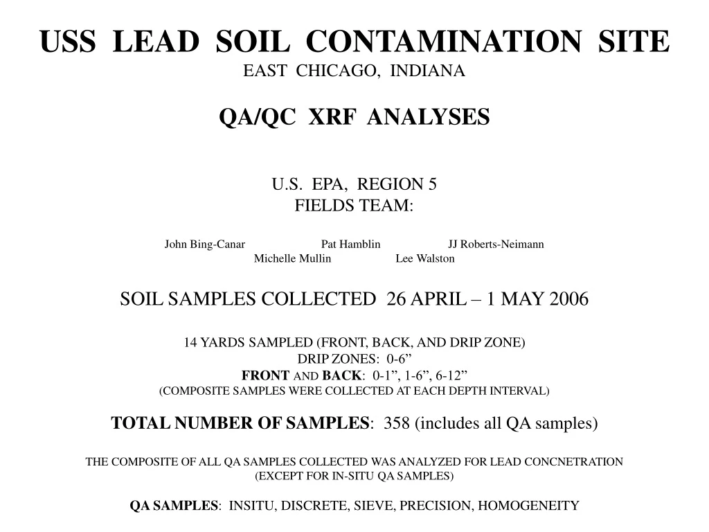
USS LEAD SOIL CONTAMINATION SITE EAST CHICAGO, INDIANA QA/QC XRF ANALYSES U.S. EPA, REGION 5 FIELDS TEAM: John Bing-Canar Pat Hamblin JJ Roberts-Neimann Michelle Mullin Lee Walston SOIL SAMPLES COLLECTED 26 APRIL – 1 MAY 2006 14 YARDS SAMPLED (FRONT, BACK, AND DRIP ZONE) DRIP ZONES: 0-6” FRONTANDBACK: 0-1”, 1-6”, 6-12” (COMPOSITE SAMPLES WERE COLLECTED AT EACH DEPTH INTERVAL) TOTAL NUMBER OF SAMPLES: 358 (includes all QA samples) THE COMPOSITE OF ALL QA SAMPLES COLLECTED WAS ANALYZED FOR LEAD CONCNETRATION (EXCEPT FOR IN-SITU QA SAMPLES) QA SAMPLES: INSITU, DISCRETE, SIEVE, PRECISION, HOMOGENEITY
RESIDENTIAL SAMPLING DESIGN Figure 1. Design for sampling residential properties in the neighborhood surrounding USS Lead.
# 1 IN SITU SAMPLES ESTIMATING SMALL-SCALE SPATIAL VARIABILITY IN SURFACE SOIL LEAD CONCENTRATIONS In-situ samples = surficial, in-situ, sampling of soil. No sample preparation. For each in-situ sample, vegetation was removed to expose surface soil. Each location was then analyzed with field-portable XRF (Niton, XLP-700) three (3) times, each measurement located within 1 inch from one another. All in-situ samples were collected at the 5-pt. locations shown in Figure 2. Thus, the total of all in-situ samples collected at each property should equal ~ 15. As with all other QA samples, analyses were performed using the XRF reported lead (Pb) concentration. COLLECTED AT A RANDOM SAMPLE OF YARDS (n = 7) X03_BACK X10_BACK X15_BACK X19_FRONT X42_FRONT X46_BACK X48_FRONT To analyze in-situ samples, the coefficient of variation (CV) was used to measure the small-scale spatial variability of lead concentrations around each sample point. The CV is the standard deviation divided by the mean, multiplied by 100 (represented as a percent). For in-situ measurements, a lower CV% indicates that there is little small-scale spatial variability. The CV was calculated zone-by-zone (A, B, C, D, or E) within each yard to measure the within-yard variability of XRF readings. The average in-situ XRF reading for lead concentration was then compared to paired composite samples at the most representative soil depth interval (0-1”) to determine if the average of in-situ XRF readings differ from 5-pt composite for each yard.
# 1 IN SITU RESULTS TABLE 1. SUMMARY STATISTICS OF IN-SITU SAMPLES ANALYZED FOR LEAD (Pb) CONCENTRATION COLLECTED AT EACH LOCATION (ZONE) Number of samples (Number) should equal 3. Some were analyzed 2 or 4 times. CV (last column) is the measure of small-scale variability. AVERAGE CV% BY YARD (± STDEV) X03: 10.2 % ± 6.5 X10: 13.0% ± 10.2 X15: 11.4% ± 7.8 X19: 6.4% ± 3.2 X42: 14.1% ± 8.0 X46: 40.6% ± 46.6 X48: 13.5% ± 7.8
# 1 IN SITU RESULTS (cont’d) Figure 2. Scatter plot of in-situ coefficient of variation (CV %) relative to XRF Pb value (ppm) for each yard analyzed (n = 7). The coefficient of variation was calculated for each zone (A, B, C, D, E). The CV% of most samples is below 30%, with the exception of two large CV% values present within yard X46.
# 1 IN SITU RESULTS (cont’d) Figure 3. Average Coefficient of Variation (CV %; ± 1 SD) of XRF lead values for each yard analyzed (n = 7). For most yards sampled, small-scale spatial variability appears to be consistent, with an overall CV % of 15.6 % (± 11.3). The inter-quartile range of CV% for all in-situ samples analyzed is between 7.3% (25th percentile) and 25.7% (75th percentile).
# 1 IN SITU RESULTS (cont’d) DO in-situ RESULTS DIFFER FROM COMPOSITES? The average of the in-situ lead values for each yard analyzed (n = 7) was compared to the composite at the most representative soil depth interval. Because in-situ samples were collected at the soil surface, they were only compared to composite samples collected at the 0-1” interval. A paired t-test was used to determine if the average in-situ value significantly differed from the paired composite value at the 0-1” interval. Natural log (ln) transformations were used to normalize the difference between in-situ and composite values. Results of this analysis revealed that there was no difference between in-situ and composite XRF values (t6 = -0.55; p = 0.60; Figure 4). On average, in-situ XRF readings were 2.3% less than composite XRF values. See Figures 4&5. Figure 4. Results of the paired t-test for ln-transformed in-situ (LOG_IN) and composite (LOG_COM) samples. Figure 5. Comparison of average in-situ and composite (0-1) XRF values for each yard analyzed.
COMPARING IN-SITU XRF SAMPLES TO LAB RESULTS USING THE AVERAGE 3-PT INSITU READING PER SAMPLE ZONE (A-E) IN-SITU XRF SAMPLES XRF AND LAB COMPOSITES AT THE 0-1”
●LAB COMPOSITE (0-1”) CONCENTRATION *XRF COMPOSITE (0-1”) CONCENTRATION The average (±1 SD) of the 5-pt insitu samples (blue boxes) with respect to paired XRF and Lab composites at the 0-1” interval.
# 2 DISCRETE SAMPLES DETERMINE SPATIAL VARIABILITY AT THE YARD-SCALE (SPATIAL UNCERTAINTY) COMPARE THE AVERAGE AND COMPOSITE OF THE DISCRETE SAMPLES DISCRETE SAMPLES = XRF measurements of each subsample from a composite to quantify spatial uncertainty within each yard. For each discrete sample, the subsample at each zone (A,B,C,D,E) was bagged and separately analyzed with XRF. Later, discrete samples were combined and an the 5-pt composite of the discrete samples was similarly analyzed. COLLECTED AT A RANDOM SAMPLE OF YARDS (n = 7) X03_BACK_0-1 X10_BACK_1-6 X15_BACK_1-6 X19_FRONT_0-1 X42_FRONT_1-6 X46_BACK_1-6 X48_BACK_1-6
# 2 DISCRETE SAMPLES (RESULTS) QUANTIFYING SPATIAL UNCERTAINTY : CV% OF DISCRETE SAMPLES CV% OF DISCRETE SAMPLES FOR EACH YARD X03: 23.0 % X10: 29.2 % X15: 23.8 % X19: 17.8 % X42: 38.9 % X46: 74.3 % X48: 55.2 % TABLE 2. Average reported lead concentration (MEAN) and spatial variability (CV%) of XRF discrete samples collected at the 5-pt locations at each yard analyzed (n = 7). COMPARING DISCRETE SAMPLES TO COMPOSITE SAMPLES Overall, there is a 12.09 % difference (magnitude, ±) between the mean and the composite of all discrete samples in each yard. On average, the XRF reading of composite samples is 9.1 %greater than the average discrete XRF reading. TABLE 3. Comparison between MEAN and the COMPOSITE of the discrete samples at each yard analyzed (n = 7).
# 2 DISCRETE SAMPLES (RESULTS) Figure 6. Spatial variability (CV%) in the average discrete samples analyzed by XRF for lead (Pb) concentration. The CV% was determined to represent spatial uncertainty at the yard-scale. There appears to be a negative relationship between CV% and the average lead concentration for the discrete samples.
# 2 DISCRETE SAMPLES (RESULTS) AT THE YARD-SCALE, THE AVERAGE CV% OF ALL DISCRETE SAMPLES IS 37.4% ± 20.5 (FIGURE 7). AT THIS SCALE, THE INTER-QUARTILE RANGE (P25 - P75) OF SPATIAL UNCERTAINTY (CV%) IS 23.0% - 55.2%. Figure 7. Average CV% (± 1 SD) of discrete samples collected from all yards analyzed (n = 7).
# 2 DISCRETE SAMPLES (RESULTS) Figure 6. Average (± 1 SD) XRF reading for DISCRETE samples analyzed for lead concentration in each yard. The average of the discrete samples (blue boxes) is denoted by the line in the center of each blue box. The length of each box is the standard deviation about the mean. The composite of all discrete samples (*) is also shown. On average, there is a 12.09 % difference between the AVERAGE and the COMPOSITE XRF value for lead concentration of the discrete samples.
# 3 SIEVED SAMPLES DETERMINING THE EFFECTS OF SIEVING ON XRF READINGS (COMPARED TO 5-PT COMPOSITE SAMPLING WITHOUT SIEVING) SIEVED SAMPLES = Randomly selected 5-pt composite samples from either the front or back yard will be analyzed before-and-after sieving. Thus, at each yard analyzed, sieved samples are compared to their paired “un-sieved” composite. COLLECTED AT A RANDOM SAMPLE OF YARDS (n = 12): X03_BACK_0-1 X07_FRONT_1-6 X10_BACK_1-6 X13_FRONT_1-6 X15_BACK_1-6 X19_BACK_1-6 X24_FRONT_1-6 X26_FRONT_1-6 X35_FRONT_1-6 X48_BACK_1-6 X49_FRONT_1-6 X50_FRONT_1-6
# 3 SIEVED SAMPLES (RESULTS) TABLE 4. XRF readings for lead concentration in SIEVED and UN-SIEVED paired composite soil samples (n = 12). OVERALL, THERE IS A 13.0 % (MAGNITUDE, ±) DIFFERENCE BETWEEN SIEVED AND UN-SIEVED COMPOSITE SOIL SAMPLES. ON AVERAGE, THE XRF READING OF SIEVED COMPOSITE SAMPLES ARE 9.2 %GREATER THAN UN-SIEVED SAMPLES. TABLE 5. Comparison between SIEVED and UNSIEVED composite soil samples (n = 12).
# 3 SIEVED SAMPLES (RESULTS) FIGURE 7. Comparison between the XRF reading for soil lead concentration (ppm) of SIEVED and UNSIEVED composite soil samples (n = 12). Most samples were analyzed at the 1-6” depth interval. Only 1 sample (X03_BACK) was analyzed at the 0-1” interval.
# 3 SIEVED SAMPLES (RESULTS) RESULTS OF THE PAIRED T-TEST THAT COMPARED XRF READING BETWEEN PAIRED SIEVED AND UN-SIEVED COMPOSITE SAMPLES. DIFFERENCES BETWEEN SIEVED AND UNSIEVED PAIRS WERE NORMALLY DISTRIBUTED, THUS, NO TRANFORMATIONS WERE NECESSARY. NO STATISTICAL DIFFERENCE (t11 = 1.89; P = 0.085) IN XRF READINGS BETWEEN SIEVED AND UN-SIEVED COMPOSITE SAMPLES. ON AVERAGE, XRF VALUES OF SIEVED SAMPLES WERE 9.2% GREATER THAN THE XRF VALUE OF UN-SIEVED SAMPLES. Mean lead concentration (± 1 SE) for each of the two sample prep methods over all sieved samples analyzed
# 4 PRECISION SAMPLES DETERMINING THE INSTRUMENT (XRF) UNCERTAINTY PRECISION SAMPLES = For each selected composite sample, 7 repeated XRF measurements are taken at the same location. The CV% of lead (Pb) concentration for these 7 repeated measurements is an indication of measurement uncertainty (the mean and SD lead concentration is also recorded). For each precision sample, the coefficient of variation (CV%) should be less than 20%, and CV% should be greater at lower lead (Pb) concentrations 1. COLLECTED AT A RANDOM SAMPLE OF YARDS (n = 11): X07_DRIP_0-6 X13_BACK_6-12 X19_BACK_6-12 X24_FRONT_1-6 X26_FRONT_6-12 X35_FRONT_1-6 X42_BACK_1-6 X46_BACK_6-12 X48_FRONT_6-12 X49_DRIP_0-6 X50_FRONT_1-6 1. Source: http://fate.clu-in.org/xrf_main.asp
# 4 PRECISION SAMPLES (RESULTS) TABLE 6. Results of the precision analyses. For each of the 11 samples, the average of the 7 repeated measures is calculated (PB_AVG). The coefficient of variation (CV%) is the measure of instrument precision / uncertainty. The coefficient of variation (CV%) was less than 20% for all precision samples analyzed (n = 11). Over all samples, the average CV% was 8.7% ± 5.9 (SD), with upper and lower 95% CL of 4.7% and 12.7% about the mean CV% (see below).
# 4 PRECISION SAMPLES (RESULTS) FIGURE 8. XRF measurement uncertainty (CV%) relative to the lead concentration analyzed. Measurement uncertainty is greater at low concentrations and decreases as lead concentrations increase.
# 5 HOMOGENIZATION ANALYSIS DETERMINING WITHIN-COMPOSITE VARIABILITY HOMOGENEITY SAMPLES = For each composite selected, 5 XRF measurements were collected, one in each corner of the bag and one in the center of the bag. The average Pb concentration of the repeated XRF measurements was calculated, and the CV% was used at the measure of within-composite variability (sample preparation uncertainty). COLLECTED AT A RANDOM SAMPLE OF YARDS (n = 10): X03_DRIP_0-6 X07_BACK_6-12 X10_DRIP_0-6 X13_BACK_1-6 X15_DRIP_0-6 X19_FRONT_0-1 X42_FRONT_6-12 X46_FRONT_1-6 X48_BACK_1-6 X49_BACK_1-6
# 5 HOMOGENIZATION SAMPLES (RESULTS) TABLE 7. For each of the 10 homogenization samples, the average of the 5 measures is calculated (PB_AVG). The coefficient of variation (CV%) is the measure of within-composite variability (sample preparation uncertainty). For the 10 homogenization samples, the coefficient of variation (CV%) was less than 20%. Over all samples, the average CV% was 12.7 % ± 12.5 (SD), with upper and lower 95% CL of 4.3% and 21.1% about the mean CV% (see below).
# 5 HOMOGENIZATION SAMPLES (RESULTS) FIGURE 9. Sample preparation uncertainty (CV%) relative to the lead concentration analyzed. Sample preparation uncertainty appears to be unrelated to the composite lead (Pb) concentration.
# 6 Comparing Pb Concentrations within Composite Samples Do XRF Readings Differ Between 0-1” and 1-6” Intervals? # 1: Analysis of Variance (ANOVA) # 2: Paired t-tests
# 6 Comparing Pb Concentrations within Composite Samples Do XRF Readings Differ Between 0-1” and 1-6” Intervals? # 1: Analysis of Variance (ANOVA) SAMPLES AND RESIDUALS WERE NORMALLY DISTRIBUTED; THUS, NO TRANSFORMATIONS WERE NECESSARY FOR ANOVA. # 2: PAIRED T-TEST SQUARE-ROOT TRANSFORMATIONS WERE USED TO NORMALIZE THE DIFFERENCES BETWEEN 0-1” AND 1-6” COMPOSITES FOR THE PAIRED T-TEST.
# 6 Comparing Pb Concentrations within Composite Samples Do XRF Readings Differ Between 0-1” and 1-6” Intervals? On average, XRF readings at the 0-1” composite sample are 5.4% [± 52.3 (SD)] greater than the composite at the 1-6”. However, due to the great amount of variability (SD=52.3 %), there is no difference in XRF reading between composite samples. MEAN ± 1 SD
PRELIMINARY CONCLUSIONS • In-Situ Samples: • Small-scale XRF readings are relatively consistent (low small-scale variability); • Average CV = 15.6 ± 11.3% (SD) for all yards sampled. • No statistical difference between In-Situ samples and composites collected at the 0-1” interval On average, In-Situ XRF readings were 2.3% less than paired composites at 0-1”. • 2. Discrete Samples • Greater level of spatial uncertainty in XRF readings at the yard-scale (greater spatial uncertainty); • Average CV (pooled across all yards) = 37.4 ± 20.5 % (SD). • 3. Sieved Samples • No statistical difference in XRF readings between Sieved and Un-sieved composite pairs. • On average, XRF readings of sieved samples were 9.2% greater than those of un-sieved pairs. • 4. Precision Samples • High level of instrument certainty (low variability) • On average, XRF precision CV = 8.7 ± 5.9% (SD). • Greater variability at low Pb concentrations than at larger Pb concentrations. • 5. Homogeneity Samples • Sample preparation uncertainty is low - XRF readings were consistent regardless of where the concentration was analyzed on the bagged composite sample • On average, XRF homogeneity CV = 12.7 ± 12.5% (SD). • For all yards analyzed, CV % was less than 20%. • Composite Samples • No difference in XRF readings between composites collected at the 0-1” and 1-6” intervals. On average, XRF readings for composites at the 0-1” interval are 5.4 ± 52.3% (SD) greater than composites at the 1-6” interval.
COMPARING XRF COMPOSITES TO LAB RESULTS N = 97 (one missing observation at X07_BACK_0-1) [5 LAB DUPLICATES – AVERAGED] Scatter plot of ‘true’ laboratory Pb concentrations vs. XRF readings
CORRELATIONS INTERVAL: 0-1” INTERVAL: 0-6” INTERVAL: 1-6” INTERVAL: 6-12” ALL SAMPLES (n = 97)
Best-Performing Linear Regression Model Weighted Least Squares Due to heteroscedasticity (greater variance at larger XRF/Lab values), a variance-stabilizing weight was applied to reduce the influence of larger, less reliable values on the model Square-root transformations of lab concentrations normalized the residuals. Lab Concentration 0.031 * (XRF Concentration) + 9.327
VERIFYING ASSUMPTIONS Due to heteroscedasticity, less weight was applied to observations where XRF value exceeds 500 ppm Square-root transformations (lab values only) normalized the residuals
Square-root Lab Conc (ppm) Regression Line With 95% Upper Confidence & Prediction Limits Square-root transformed LAB CONC Weighted least squares regression line ( ) for predicted laboratory concentrations. The 95% upper confidence (---) and prediction ( ) intervals are also shown.
Regression Line With 95% Upper Confidence & Prediction Limits BACK-TRANSFORMED LAB CONC
Do Lead Concentrations Differ at Depth? (Do concentrations decline at deeper intervals?) USS Lead Soil Contamination Site 05 March 2007 X07 Backyard was only sampled at 1-6” and 6-12” intervals; thus, this yard (X07_B) was omitted from analysis. All remaining yards (N = 27) were sampled at the 0-1”, 1-6”, and 6-12” intervals; Drip zone samples were omitted from this analysis.
Do Lead Concentrations Differ at Depth? (Do concentrations decline at deeper intervals?) USS Lead Soil Contamination Site 05 March 2007 TESTING ASSUMPTIONS FOR PARAMETRIC STATISTICS Tests for Normality S-W: W=0.902; P<0.001 K-S: D=0.096; P=0.064 A-D: A=1.264; P=0.005 Raw Data Analytical Results CONCENTRATIONS ARE NOT NORMALLY DISTRIBUTED
Do Lead Concentrations Differ at Depth? (Do concentrations decline at deeper intervals?) USS Lead Soil Contamination Site 05 March 2007 TESTING ASSUMPTIONS FOR PARAMETRIC STATISTICS Tests for Normality S-W: W=0.936; P<0.001 K-S: D=1.58; P=0.010 A-D: A=2.231; P<0.001 LN-Transformed Data Analytical Results CONCENTRATIONS ARE NOT NORMALLY DISTRIBUTED
Do Lead Concentrations Differ at Depth? (Do concentrations decline at deeper intervals?) USS Lead Soil Contamination Site 05 March 2007 TESTING ASSUMPTIONS FOR PARAMETRIC STATISTICS Tests for Normality S-W: W=0.969; P=0.051 K-S: D=0.081; P=0.150 A-D: A=0.750; P=0.050 Square-Root Transformed Data Analytical Results CONCENTRATIONS ARE NORMALLY DISTRIBUTED
Do Lead Concentrations Differ at Depth? (Do concentrations decline at deeper intervals?) USS Lead Soil Contamination Site 05 March 2007 Only square-root transformed analytical lead concentrations were normally distributed and were included in the Analysis of Variance (ANOVA) model to determine if concentrations differed among soil depth intervals. Full-factorial, balanced design: 1 Independent Variable (Depth Interval) - 3 levels: a. 0-1” b. 1-6” c. 6-12” Each level contained equal observations of the dependent variable (square-root lab concentrations) Due to the balanced design, Type I sums of squares were used in the ANOVA model. Levene’s test for homogeneity of error variances Tukey-Kramer post-hoc test for differences among groups Output dataset with residuals to determine if residuals are normally distributed
Do Lead Concentrations Differ at Depth? (Do concentrations decline at deeper intervals?) USS Lead Soil Contamination Site 05 March 2007 ANOVA RESULTS There is a difference in transformed concentrations among the three intervals F2,78 = 9.28; P < 0.001 Assumption of homogeneity of error variances is met. Variances are NOT heteroscedastic (P = 0.972) (See the box plots on the next slide)
Do Lead Concentrations Differ at Depth? (Do concentrations decline at deeper intervals?) USS Lead Soil Contamination Site 05 March 2007 Box Plot of square-root transformed lead concentrations among the 3 soil depth intervals. This plot shows that the variability (bars) are nearly consistent at each interval, supporting the Levene’s Test for homogeneity of error variances. TESTING ASSUMPTIONS: Homogeneity of the error variances Error variances are equal across groups
Do Lead Concentrations Differ at Depth? (Do concentrations decline at deeper intervals?) USS Lead Soil Contamination Site 05 March 2007 TESTING ASSUMPTIONS: Normality of the Residuals Tests for Normality S-W: W=0.984; P=0.411 K-S: D=0.057; P=0.150 A-D: A=0.301; P=0.250 Square-Root Transformed Data Residuals RESIDUALS ARE NORMALLY DISTRIBUTED
Do Lead Concentrations Differ at Depth? (Do concentrations decline at deeper intervals?) USS Lead Soil Contamination Site 05 March 2007 TUKEY – KRAMER POST HOC TEST No difference between 0-1” and 1-6” (P = 0.990) Concentrations at 6-12” are different from both 0-1” and 1-6” (P< 0.0013)
Do Lead Concentrations Differ at Depth? (Do concentrations decline at deeper intervals?) USS Lead Soil Contamination Site 05 March 2007 Bar chart of mean (average) square-root transformed lead concentrations among the three soil depth intervals. Error bars rerpresent ± 1 standard error (SE). This chart shows that concentrations at the 6-12” interval are less than the concentrations at the 0-1” and 1-6” intervals; there is no difference in concentrations at the 0-1” and 1-6” intervals.
Do Lead Concentrations Differ at Depth? (Do concentrations decline at deeper intervals?) USS Lead Soil Contamination Site 05 March 2007 Non-Parametric ANOVA by Ranks Test Dependent variable (lab concentration) was rank-transformed prior to analysis; this analysis is non-parametric, thus no assumptions about the data are required to be met. Consistent with the parametric ANOVA model, this non-parametric ANOVA by Ranks Test indicates that there is a difference in lead concentration among the depth intervals (F2,78 = 8.93; P < 0.001). Furthermore, the Tukey HSD test indicated that only concentrations at the 6-12” interval were different than the concentrations at the other intervals; there was no difference in concentrations at the 0-1” and 1-6” intervals.
Do Lead Concentrations Differ at Depth? (Do concentrations decline at deeper intervals?) USS Lead Soil Contamination Site 05 March 2007