Load Balancing Myths, Fictions & Legends

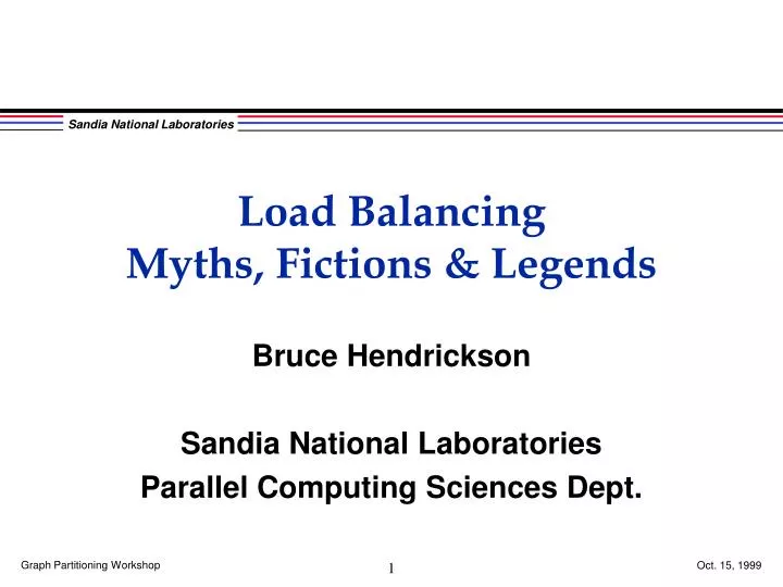
1. Load BalancingMyths, Fictions & Legends Bruce Hendrickson Sandia National Laboratories Parallel Computing Sciences Dept. 1

2. Introduction • Two happy occurrences. • (1) Good graph partitioning tools & software. • (2) Good parallel efficiencies for many applications. • Is the latter due to the former? • Yes, but also no. • We have been lucky! • Wrong objectives. • Models insufficiently general. • Software tools often poorly designed. 2

3. Myth 1:The Edge Cut Deceit • Generally believed that “Edge Cuts = Communication Cost”. • This assumption is behind the use of graph partitioning. • In reality: • Edge cuts are not equal to communication volume. • Communication volume is not equal to communication cost. 3

4. Edge Cuts Versus Volume Edge cuts = 10. Communication volume: 8 (from left partition to right partition). 7 (from right partition to left partition). 4

5. Communication Volume • Assume graph edges reflect data dependencies. • Correct accounting of communication volume is: • Number of vertices on boundary of partition. • Elegant alternative is hypergraph model of Çatalyürek, Aykanat, Pinar and Pinar. • Volume is number of cut hyperedges. 5

6. Communication Cost • Cost of single message involves volume and latency. • Cost of multiple messages involves congestion. • Cost within application depends only on slowest processor. • Our models don’t optimize the right metrics! 6

7. Why DoesGraph Partitioning Work? • Vast majority of applications are computational meshes. • Geometric properties ensure that good partitions exist. • Communication/Computation = n1/2 in 2D, n2/3 in 3D. • Runtime is dominated by computation. • Vertices have bounded numbers of neighbors. • Error in edge cut metric is bounded. • Homogeneity ensures all processors have similar subdomains. • No processor has dramatically more communication. • Other applications aren’t so forgiving. • E.g. Interior point methods, latent semantic indexing, etc. • We have been lucky! 7

8. Myth 2: Simple Graphs are Sufficient • Graphs are widely used to encode data dependencies. • Vertex weights reflect computational cost. • Edge weights encode volume of data transfer. • Graph partitioning determines data decomposition. • However, many problems are not easily expressed this way! • Complex relationships or constraints on partitioning. • E.g. computation on nodes and on elements. • DRAMA has a uniquely rich model for this problem. • Dependencies are directed (e.g. unsymmetric matvec). • Computation consists of multiple phases. 8

9. Alternative Graph Models • Hypergraph model (Aykanat, et al.) • Vertices represent computations. • Hyperedge connects all objects which produce/use datum. • Handles directed dependencies. • Bipartite graph model (H. & Kolda) • Directed graph replaced by equivalent bipartite graph. • Handles directed dependencies. • Can model two-phase calculations. • Multi-Objective, Multi-Constraint (Schloegel, Karypis & Kumar) • Each vertex/edge can have multiple weights. • Can model multiple-phase calculations. 9

10. Myth 3: Partition Quality is Paramount • Partitioners compete on edge cuts • and (sometimes) runtime. • This isn’t the full story • particularly for dynamic load balancing! 10

11. 7 Habits of Highly Effective Dynamic Load Balancers • Balance the load • Balance each phase or some combination? • How is load measured? • Minimize communication cost • Volume? Number of messages? Something else? • Run fast in parallel • Be incremental • Make new partition similar to current one • Not use too much memory • Support determination of new communication pattern • Be easy to use 11

12. Performance Tradeoffs • From Touheed, Selwood, Jimack and Berzins. • ~1 million elements with adaptive refinement. • 32 processors of SGI Origin. • Timing data for different partitioning algorithms. • Repartitioning time per invocation: 3.0 - 15.2 seconds. • Migration time per invocation: 17.8 - 37.8 seconds. • Explicit solve time per timestep: 2.54 - 3.11 seconds. • Observations: • Migration time more important than partitioner runtime. • Importance of quality depends on: • Frequency of rebalancing. • Cost of solver. 12

13. Myth 4: Existing Tools Solve the Problem • Lots of good software exists. • Static partitioning is fairly mature. • However, it addresses an imperfect model. • Dynamic partitioning is more complicated. • Applications differ in need for cost, quality or incrementality. • No algorithm is uniformly best. • Good library should support several (e.g. DRAMA). • Subroutine interface requires good software engineering. • E.g. Zoltan?. 13

14. Myth 5: The Key is Finding the Right Partition • Assignment of work to processors is the key to scalability. • However, this needn’t be a single partition. • Example: parallel crash simulations. • In each timestep: • (1) Do finite element analysis & predict new deformations. • (2) Search for grid intersections (contact detection). • (3) If found, correct deformations & forces. • Each stage has different objects & different data dependencies. • Very difficult to balance them all with one decomposition. • But most work on this problem has taken this approach. 14

15. Multiple Decompositions • Finite element analysis: • Topological • Static • Contact detection: • Geometric • Dynamic • Key Idea: • Use graph partitioning for finite element phase • Use geometric partitioner for contact detection • We use recursive coordinate bisection (RCB) 15

16. Parallel Crash Simulations • Outline of parallel timestep in Pronto code: • 1. Finite element analysis in static, graph-based decomposition. • 2. Map contact objects to RCB decomposition. • 3. Update RCB decomposition. • 4. Communicate objects crossing processor boundaries. • 5. Each processor searches for contacts. • 6. Communicate contacts back to finite element decomposition. • 7. Correct deformations, etc. • Observations: • Reuse serial contact software. • RCB is incremental & facilitates determination of communication. • Each phase should scale well. • Cost of mapping between decompositions? 16

17. Can Crush Example RCB Decomposition as can gets crushed RCB on undeformed geometry Finite element decomposition 17

18. Scalability • Can crush problem, 3800 elements per compute node, run to 100 ms.A 13.8-million element simulation on 3600 compute nodes ran at 0.32 seconds per time step (120.4 Gflops/s). overhead contacts FEM 18

19. Micro-mechanics of Foam 19

20. Myth 6:All the Problems are Solved • Biggest & most damaging myth of all! • Already discussed need for: • More accurate & expressive models. • Algorithms for partitioning new models. • More user-friendly tools. • Lots of other open problems. 20

21. Open Problems • Partitioning for multiple goals. • Examples: • Multiple phases in a calculation. • Minimize communication volume and number of messages. • Multi-objective/constraint work is partial answer. • Only models costs on graph vertices or edges. • Can’t minimize number of messages. • New ideas are needed. • Partition to balance work of sparse solve on each subdomain. • Applications to FETI preconditioner, parallel sparse solvers, etc. • Complicated dependence on topology of submesh. • Can’t predict cost by standard edge/vertex weights. 21

22. More Open Problems • Partitioning for heterogeneous parallel architectures. • E.g. Clusters of SMPs, Beowulf machines, etc. • How to model heterogeneous parallel machines? • How to adapt partitioners to address non-standard architectures? • (See Teresco, Beall, Flaherty & Shephard.) • Partitioning to minimize congestion. • Communication is limited by most heavily used wire. • How can we predict and avoid contention for wires? • (See Pellegrini or H., Leland & Van Driessche.) 22

23. More Information • Contact info: • bah@cs.sandia.gov • http://www.cs.sandia.gov/~bahendr • Collaborators: • Rob Leland Karen Devine Tammy Kolda • Steve Plimpton Bill Mitchell • Work supported by DOE’s MICS program • Sandia is a multiprogram laboratory operated by Sandia Corporation, a Lockheed-Martin Company, for the US DOE under contract DE-AC-94AL85000 23