Download
1 / 23
260 likes | 645 Views
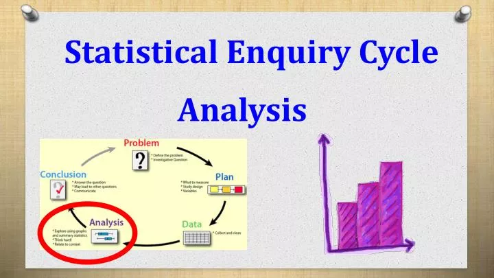
Statistical Enquiry Cycle Analysis. What the Analysis stage involves. Calculation of Summary Statistics Calculation of Informal Confidence Intervals Drawing of Comparative Dot Plots, Box & Whisker Plots I notice statements… Central Tendency, Unusual Values, Shape, Shift, Spread

E N D
What the Analysis stage involves • Calculation of Summary Statistics • Calculation of Informal Confidence Intervals • Drawing of Comparative Dot Plots, Box & Whisker Plots • I notice statements… • Central Tendency, Unusual Values, Shape, Shift, Spread • Minimum of 3 • Must be comparative • Must be contextual • Based on your samples – could you make predictions for population (statistical insight)
What the Analysis stage involves (cont) • Statistical Inference • Using your informal confidence intervals, state what you think the population medians for each group is likely to be • Make a statement regarding overlap, and what this means in regards to back in the population
Summary Statistics You are required to calculate the following, either manually or via calculator
What is Standard Deviation?? Standard Deviation (s.d.) is a measure of the average spread of numbers from the mean. Like the mean, it is a formal mathematical calculation. It also suffers like the mean, by the influence of outliers and extreme values. A sample with a low s.d. has data that is less spread out than a sample with a larger s.d. Approximately 68% of data values are within 1 s.d. of the mean. Approximately 95% of data values are within 2 s.d. of the mean. Mean (x̅)
Informal Confidence Intervals Due to sampling variability, we cannot be certain of providing an accurate estimate of the population median. Therefore we provide a range of values, or an interval within which the population median probably lies. This interval is known as a Confidence Interval. The question is, how confident am I that my population Median lies in the interval provided by my sample? 95%
Calculation of Informal Confidence Intervals The range that the Population Median will lie in 95% of the time - Decreases when sample size increases - Increases when spread increases Putting this all together gives us the range of medians The interval created by this process is called an informal confidence interval for the population median.
Displaying the confidence interval on box plots It is shown on the box plot by a clear defined horizontal line extending from the median All graphs to be clearly labelled
I notice statements These areas require your analysis: comparative and contextual! C– central tendency – look at the data’s, mean, median, and mode – use visible information from boxplot to help U – unusual values – are there any, if so, make statements (if not state this) – look at dot plot, identify and comment upon S – spread – look at range, the IQR (the box – the middle 50%) and standard deviation S– shape – what is the symmetry like (even, or skewed?) – modal, bimodal or no mode – distribution of data (normal, uniform, or other)
I notice statements S– shift – from the boxplot, has one box (middle 50%) moved up the scale in relation to the other box (middle 50%). Also consider whole data as well. So these 5 things are what you need to describe using “I notice…” statements, using numerical and contextual evidence to support it. CUSSS – remember it!
Central Tendency Comparing measures of central tendency MEDIAN: directly from the boxplots MEAN: directly from the summary statistics (remember it is a mathematical average, therefore affected by outliers) “…median of those who survived (2.2kg) is greater than those who died (1.6kg)… “…median of guesses for the fall (252), did not differ much to the median of the guesses for the spring (255)… What could you imply about the population median based on your samples?
Unusual Values Are there any? If so, decide, are they outliers or extremes? I notice that from the dot plot for males, one student who had 18 pairs of shoes. I would classify this as an outlier, in comparison to the rest of the males data. I notice that males have an extreme value at 110, and females have two extreme values at 108 and 122. Would your population experience unusual values likes these?
Boxplot showing outliers, and extreme values Outliers are values that lie outside 1.5 x IQR, but within 3 x IQR Extreme values lie outside 3 x IQR Whiskers extend to the highest value within 1.5 IQR The same applies to the lower end values
Spread What do you notice about the spread of the data? RANGE: discuss, as a simple statement, (if outliers are present the range would be smaller if they were excluded (reason why?)) IQR: more important to discuss. Is one clearly larger than the other, or similar in size – what does this mean in the context of the data? STANDARD DEVIATION: compare for both groups – what does it mean? I notice that the IQR for boys right-foot length(XX cm) is much smaller than that for girls (YY cm). This could be due to … I notice that the IQR for the boys armspan (XX cm) is very similar to that for girls (YY cm). This is because… What could you imply about the spread for your groups back in the population?
Shape Dot Plot graphs: Comment on both datasets, some common ones are shown below. A symmetric distribution is one that shows symmetry about its centre. Both normal and rectangular (uniform) distributions show symmetry, and some bimodal distributions can as well. Remember – this is related to how spread the data is What could you expect the same kind of shape in the population? Why?
Shape Boxplot graphs, what do you notice about Overall shape: - are the length of the whiskers the same length? - if yes, then you can say the overall distribution shows overall symmetry - if no, then overall there is some skewness present Middle 50% shape: - is the median in the middle of the box - if yes, then you can say the middle 50% is symmetrical -if no, then there is some skewness within the middle 50% of the data
Shift This relates to where the box (middle 50%) of one set of data is in relation to the box (middle 50%) of the comparative set of data. I notice that the age of the chess players is shifted towards older ages than the age of the badminton players. This is shown by the middle 50% of chess players ages being higher (or shifted towards higher ages) than for the middle 50% of badminton players. I also notice that the lower 75% of badminton player ages is below the top 50% of the chess player ages.
Informal Confidence Intervals Male: [27,37] Female: [29,44] NOTE: Discussion of what each informal confidence interval means (in context & referring back to the population, and how sure you are) Males:From the informal confidence interval, I am reasonably confident that the median number of hours worked for the male population is between 27 and 37 hours of work per week. Females:From the informal confidence interval, I am reasonably confident that the median number of hours worked for the female population is between 29 and 44 hours of work per week.
Statistical Inference How can we use the confidence intervals to help make a decision on whether there is a difference between the two population means (or medians) to draw a conclusion? Is there an overlap between the informal confidence intervals? How does Population A compare to Population B?
Informal Confidence Intervals - inference Male: [27,37] Female: [29,44] NOTE: Discussion of what each informal confidence overlap / or not (in context & referring back to the population and how sure you are) Because these informal confidence intervals overlap, we have no evidence that suggests the median hours worked per week for males is different from the median hours worked per week for females.
Statistical Inference You must make an inference, which will be a conclusion about the population medians based on their samples taken from the population. Your conclusion will answer the posed investigative question and will involve making a call about the population medians. The informal confidence intervals will be used to make an inference about the population medians.
Summing Up • Due to sampling variability, different samples will give different informal confidence intervals for the population median • However, about 90% of the intervals constructed in this way will contain the actual value of the population median • This means that it is a fairly safe bet that the population median lies inside the confidence interval