Download

1 / 27
270 likes | 373 Views
A multiobjective parallel machine problem considering eligibility and release and delivery times. Manuel Mateo manel.mateo@upc.edu Departament Organització d’Empreses, Universitat Politècnica Catalunya. Barcelona (Spain). HAROSA, Barcelona (14/06/12). Summary. Introduction: the real case

E N D
A multiobjective parallel machine problem considering eligibility and release and delivery times Manuel Mateo manel.mateo@upc.edu Departament Organització d’Empreses, Universitat Politècnica Catalunya. Barcelona (Spain) HAROSA, Barcelona (14/06/12)
Summary • Introduction: the real case • Scheduling of jobs The multiobjective problem • Problem Pm/rj,qj,Mj/(Cmax,W) • State of the art • A biobjective problem, the Pareto front • Algorithm • Computational experiments • Computational experience • Conclusions
Introduction: the real case (I) • The manufacturing of products is usually divided in operations or phases of transformation. • Usually one of them becomes the bottleneck of the process. • In the presented problem, we suppose this bottleneck is an intermediate phase. • Therefore, some operations are done before (the total time to work them out leads to a release time) and some others are done after (their total time is called delivery or queue time). release times bottleneck queue times
Introduction: the real case (II) • Manufacturing plants usually have several machines or assembly lines. • There are several products to be manufactured. • A usual situation is a product is assigned to a machine (line) and will be only manufactured in that machine. Line 1 INITIAL SITUATION Line 2 Line 3 2 l 1 l 50cl 33cl Line 4
Introduction: the real case (III) • Nevertheless, there could be more product-machine assignments according to capabilities of the machines. High-level machines 1 l 50cl 33cl Line 1 2 l 1 l 50cl 33cl Medium-level machines Line 2 CONSIDERED SITUATION 2 l Med.- level High- level Low- level 1 l 50cl 33cl Line 3 2 l Low-level machines 1 l 50cl 33cl Line 4 2 l
Introduction: the real case (IV) • The managers prefer the use of the most modern resources (high-level machines). But if all the jobs were done in these machines, the makespan would be very high. The rest of machines would be completely free. • Some works from machines of the high-level are moved to the other machines. • Machinery for reduced products is considered in the low-level. • The medium-level machines can work the reduced products and also others. They are preferred to the low-level machines. • We define a penalty or weight for job j: • wj=1 if a job (of medium-level or low-level) is scheduled in a medium-level machine; • wj=2 if a job (of low-level) is scheduled in a low-level machine.
Scheduling of jobs (I) A set of n jobs (j=1,…,n) to be scheduled on m parallel machines (i=1,…,m) Given a job j, it is known: • the processing time pjfor the operation, • the release time rj(also called head times), • the delivery or queue time qj(also tail times), • the associated level lj. The machines are distributed among p groups or levels (k=1,…,p). • Particularly, we propose an algorithm for p=3 (high-level, medium-level and low-level). • Any machine i and job j is classified into one of the levels. • A machine associated to a level k can produce jobs of its own level and from a lower level. • The processing time of a job is the same for any machine.
0 t Scheduling of jobs (II) For a job of any level: high (h), medium (m) or low (l) • The release times (rj) and the delivery times (qj) are considered due to the initial availability of the job and the necessary subsequent tasks. • After the delivery time, the job is considered finished (completion time, cj). • Setup times and pre-emption are not considered. cj
Problem Pm | rj,qj,Mj | (Cmax ,Wtot) • Objective: find a feasible schedule (where j includes the assigned machine and the start time of job j) of minimum completion time (cmax) and minimum total penalization (W). • Given tjthe starting time for the job j: ; the makespan is determined: • Given xjthe machine level where the job j is assigned, the weight for the job j is: wj=xj-1 and the total weight is determined: • A schedule is feasible if the next conditions are accomplished: • Each machine processes at most one job at a time. • A job is only processed in a single machine. • Pre-emption is not allowed. • Starting time is not lower than the release time: • A job of level k is processed in a machine of the same level or a higher level.
HL HL ML ML LL LL t 0 t 0 Problem Pm | rj,qj,Mj | (Cmax ,Wtot) Machines Jobs High-level High-level Medium-level Medium-level Low-level Low-level Wtot=0 Wtot=8
Example 1 Wtot (14;6) Max Wtot (36;0) Min Wtot Cmax Min Cmax Max Cmax
Basis for the main algorithm • Gharbi, A; Haouari, M. (2002). Minimizing makespan on parallel machines subject to release dates and delivery times. Journal of Scheduling; vol. 5; pp. 329-355. • It considers release and delivery times. • Problem without considering eligibility • It is the base for solving the problem (for mk>1) Methodology • Classification of the jobs into 3 groups. • Scheduling of the 3 groups of jobs: • Scheduling of jobs with medium qj and rj values ( ) • Scheduling of jobs with low qj values ( JQ ) • Scheduling of jobs with low rjvalues ( JR ) Condition 1: Condition 2:
Generating a sub-solution per level: • Heuristics • Gharbi & Haouari (2002) Basis for the main algorithm (II) Scheduling at each level Selection of a job to be moved between levels • Which one to select? According to processing, release, queue times or an addition of these? Sequence of changes between levels • Initial tests: High-medium, high-low, medium-low
The best of both solutions Scheduling Algorithm (I) Generating a sub-solution per level Heuristic 1 Heuristic 2 is a job of the set J such that or corresponds to is a job of the set J such that or corresponds to 1 1 release time first position; else, last position release time last position; else, first position 2 2 3 3 If , end; else, Step 1 If , end; else, Step 1
ml t 0 10 20 25 30 5 15 Scheduling Algorithm (II) Example 1: ml=1 j10 j9 j7 j11 j8
Step 0.1: Initialization Step 0.2: Condition 1. If there is no job; Step 0.3. If not: Step 2.1: Assignment of jobs such that j Update u0 Step 2.3: Assignment of jobs such that j Update u0 Step 2.2: Invert scheduling Step 2.4: Invert scheduling Step 0.3: Condition 2. If there is no job, Step 0.4. If not: Step 1: Assignment of jobs such that j Scheduling Algorithm (III) Generating a sub-solution per level Step 0.4: If there are no changes in Step 0.3, STOP. If not, Step 0.2. Process Gharbi & Haouari (2002) Pre-process
ml1 j7 ml2 j9 j11 j8 0 10 20 5 15 Scheduling Algorithm (IV) Example 2 (algorithm of Gharbi & Haouari): ml=2 Step 1 Step 1 Step 2 10
How to face the multiobjective problem? • At the beginning, all the jobs are scheduled in the high-level machine(s), as they are the preferred machines to manufacture any product. • This can induce a relative high Cmax. • Then, in order to improve this value, some of the jobs are moved from a level to another lower level. In this way, the orders can be finished in a lower Cmax. • The changes between adjacent levels will be denoted by a weight =1, i.e. between high and medium level and between medium and low level, and a weight = 2, i.e. between high and low level. • Therefore, the algorithm gives different solutions, characterized by two objectives: • Min {Cmax} • Min {W}
Main Algorithm • Basically the algorithm is divided in the following phases: • PHASE I. All the jobs are scheduled in the high-level machines. If mh=1, apply Heuristic 1 for all the jobs. Otherwise, apply Heuristic 2 for all the jobs. Compute Cmaxº This implies the first solution s1=(Cmax0; Wtot0=0) • PHASE II. While Cmax can be reduced: a) select a job to be changed to a different level (only a subset of jobs are available); b) the origin level of the movement is predetermined; the destination level should be selected. Machines in both levels will be re-scheduled. This leads to a new solution sz=(Cmaxz; Wtotz)
Main Algorithm (II) PHASE II: Movement of jobs between different levels • II.1. Job movement from high to medium level Compute the new solutions (Cmax, CmaxH, CmaxM) • II.2. Job movement from high to low level Compute the new solutions (Cmax, CmaxH, CmaxL) • II.3. Job movement from medium to low level Compute the new solutions (Cmax, CmaxM, CmaxL)
Main Algorithm (III) II. Job movement from a level to a lower level Given the previous solution s (Cmaxs; Wtots) and Cmaxº= Cmaxs Briefly, the substeps in this phase are: • Select the origin level of the movement is given (here is prefixed). • Select a job to be changed to a different level (only a subset of jobs is available): Search for job candidates: JC Select a job between the candidates according to a prefixed rule (j*JC) • Select the destination level of the movement (here is prefixed). • Reschedule jobs in both levels. • Compute both objectives of the new solution (Cmax; Wtot). • IF Cmax < Cmaxº save the new solution (Cmaxs+1=Cmax ; Wtots+1=Wtot) Cmaxº=Cmax
Computational experience • To check the efficiency of the algorithm, a set of instances similar to those used by Gharbi & Haouari (2002) are created: • # jobs (n = 20) • 100 instances • Jobs of high level, 20-30% of the total number; medium level, 20-50% of the total; low level, the rest (20-60% of the total) • # machines (m = 4, 5, 6) • Processing time: discrete uniform distribution . • Release and delivery times: discrete distribution . K=3,5
Computational experience. Rules • Given the subset of candidates (considering the origin and destination levels), different rules are used to select the job to be reassigned: Consider the processing time and the other times (release and queue) j = argminj (rj+pj, qj+pj) min(rp,qp) j = argmaxj (rj+pj, qj+pj) max(rp,qp) Consider the other times (release and queue) j = argminj (rj, qj) min(r,q) j = argmaxj (rj, qj) max(r,q) Consider only the processing time j = argminj (pj) min(p) j = argmaxj (pj) max(p)
Comparison of results v1 (rule selection) • Given the solutions in the Pareto front with two different rules A and B for the job selection: • Proportion of non-dominated solutions (overall 13 distributions)
Results v1 (analysis by machines) • Proportion of non-dominated solutions for max(p) rule depending on the number of machines per level
Conclusions • In the first situation all the jobs are assigned to machines of the high level; this solution shows a great cmax with wtot=0. • The rest of solutions in the Pareto front have a decreasing cmax while wtot increases. • Different rules are tested to select a job to be moved from a level to another. • The best results are achieved with the max(pj), although the rule max(rj+pj,qj+pj) has also a good performance. • About the current and future research: • Select the origin level of job movement (level in which there is the machine with the highest Cmax). • Use of metaheuristics.
A multiobjective parallel machine problem considering eligibility and release and delivery times Thank you for your attention!