Download
1 / 17
180 likes | 283 Views
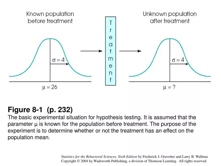
Figure 8-1 (p. 232) The basic experimental situation for hypothesis testing. It is assumed that the parameter µ is known for the population before treatment. The purpose of the experiment is to determine whether or not the treatment has an effect on the population mean.

E N D
Figure 8-1 (p. 232) The basic experimental situation for hypothesis testing. It is assumed that the parameter µ is known for the population before treatment. The purpose of the experiment is to determine whether or not the treatment has an effect on the population mean.
Figure 8-2a (p. 234) Two views of the general research situation. From both perspectives a treatment is administered to a sample and the treated sample can be compared with the original, untreated population.l The hypothesis test is concerned with the unknown population that would exist if the treatment were administered to the entire population.
Figure 8-3 (p. 236) The set of potential samples is divided into those that are likely to be obtained and those that are very unlikely if the null hypothesis is true.
Figure 8-4 (p. 238)The critical region (very unlikely outcomes) for = .05.
Table 8-1 (p. 244)Possible outcomes of a statistical decision.
Figure 8-5 (p. 245) The locations of the critical region boundaries for three different levels of significance: = .05, = .01, and = .001.
Figure 8-6 (p. 247) The structure of a research study to determine whether prenatal alcohol affects birth weight.
Figure 8-7 (p. 248)Locating the critical region as a three-step process. You begin with the population of scores that is predicted by the null hypothesis. Then, you construct the distribution of sample means for the sample size that is being used. The distribution of sample means corresponds to all the possible outcomes that could be obtained if H0 is true. Finally, you use z-scores to separate the extreme outcomes (as defined by the alpha level) from the high-probability outcomes. The extreme values determine the critical region.
Figure 8-8 (p. 250)Sample means that fall in the critical region (shaded areas) have a probability less than alpha (p < ). H0 should be rejected. Sample means that do not fall in the critical region have a probability greater than alpha (p > ).
Figure 8-9 (p. 254)The distribution of sample means for n = 16 if H0 is true. The null hypothesis states that the diet drug has no effect, so the population mean will be 10 or larger.
Figure 8-11 (p. 262) The appearance of a 15-point treatment effect in two different situations. In part (a), the standard deviation is σ = 100 and the 15-point effect is relatively small. In part (b), the standard deviation is σ = 15 and the 15-point effect is relatively large. Cohen’s d uses the standard deviation to help measure effect size.
Figure 8-12 (p. 265)The distribution of sample means for a population with a hypothesized mean of µ = 200. Notice that the critical region, determined by = .05, is shown by shading the entire area beyond z = 196 and z = –1.96
Figure 8-13 (p. 266) The null distribution and critical region from Figure 8.12, and a treatment distribution showing the set of sample means that would be obtained with a 20-point treatment effect. Notice that the null distribution is centered at µ = 200 (no effect) and the treatment distribution is centered at µ = 220 (showing a 20-point effect). Also notice that with a 20-point effect, more than 50% of the sample means would be in the critical region and would lead to rejecting the null hypothesis.
Figure 8-14 (p. 267) The null distribution and critical region from Figure 8.12, and a treatment distribution showing the set of sample means that would be obtained with a 40-point treatment effect. Notice that the null distribution is centered at µ = 200 (no effect) and the treatment distribution is centered at µ = 240 (showing a 40-point effect). Also notice that with a 40-point effect, nearly all of the possible sample means would be in the critical region and would lead to rejecting the null hypothesis.
Figure 8-15 (p. 268)The relationship between sample size and power. The top figure (a) shows a null distribution and a 20-point treatment distribution based on samples of n = 16 and a standard error of 10 points. Notice that the right-hand critical boundary is located in the middle of the treatment distribution so that roughly 50% of the treated samples fall in the critical region.In the bottom figure (b) the distributions are based on samples of n = 100 and the standard error is reduced to 4 points. In this case, essentially all of the treated samples fall in the critical region and the hypothesis test has power of nearly 100%.