Download
1 / 38
380 likes | 383 Views
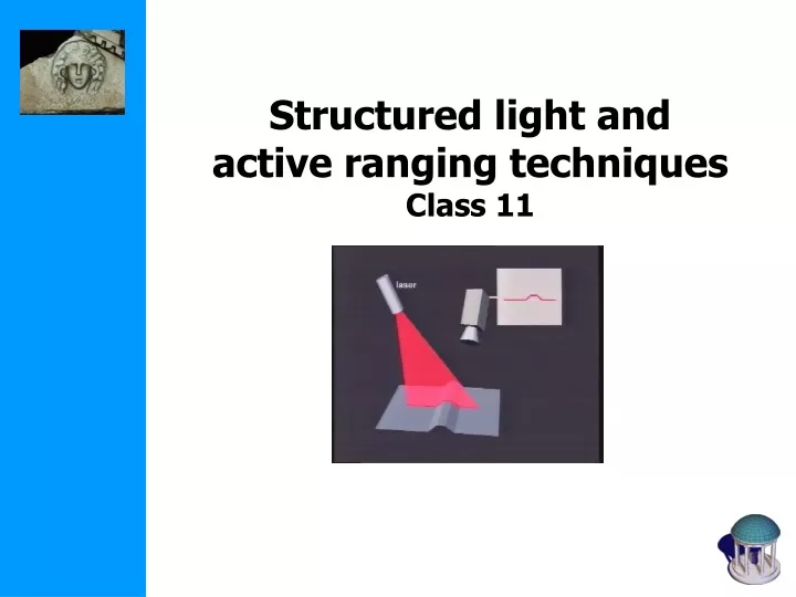
Structured light and active ranging techniques Class 11. last Tuesday: stereo. per-pixel optimization. per-scanline optimization. full image optimization. original image pair. planar rectification. polar rectification. Plane-sweep multi-view matching.

E N D
last Tuesday: stereo per-pixel optimization per-scanline optimization full image optimization
original image pair planar rectification polar rectification
Plane-sweep multi-view matching • Simple algorithm for multiple cameras • No rectification necessary, but also no gain • Doesn’t deal with occlusions Collins’96; Roy and Cox’98 (GC); Yang et al.’02/’03 (GPU)
Today’s class • unstructured light • structured light • time-of-flight (some slides from Szymon Rusinkiewicz, Brian Curless)
Unstructured light project texture to disambiguate stereo
Space-time stereo Davis, Ramamoothi, Rusinkiewicz, CVPR’03
Space-time stereo Davis, Ramamoothi, Rusinkiewicz, CVPR’03
Space-time stereo Zhang, Curless and Seitz, CVPR’03
Space-time stereo Zhang, Curless and Seitz, CVPR’03 • results
Triangulation: Moving theCamera and Illumination • Moving independently leads to problems with focus, resolution • Most scanners mount camera and light source rigidly, move them as a unit
Triangulation: Moving theCamera and Illumination (Rioux et al. 87)
Laser Camera Triangulation: Extending to 3D • Possibility #1: add another mirror (flying spot) • Possibility #2: project a stripe, not a dot Object
Triangulation Scanner Issues • Accuracy proportional to working volume(typical is ~1000:1) • Scales down to small working volume(e.g. 5 cm. working volume, 50 m. accuracy) • Does not scale up (baseline too large…) • Two-line-of-sight problem (shadowing from either camera or laser) • Triangulation angle: non-uniform resolution if too small, shadowing if too big (useful range: 15-30)
Triangulation Scanner Issues • Material properties (dark, specular) • Subsurface scattering • Laser speckle • Edge curl • Texture embossing
Space-time analysis Curless ‘95
Space-time analysis Curless ‘95
Multi-Stripe Triangulation • To go faster, project multiple stripes • But which stripe is which? • Answer #1: assume surface continuity e.g. Eyetronics’ ShapeCam
Real-time system Koninckx and Van Gool
Multi-Stripe Triangulation • To go faster, project multiple stripes • But which stripe is which? • Answer #2: colored stripes (or dots)
Multi-Stripe Triangulation • To go faster, project multiple stripes • But which stripe is which? • Answer #3: time-coded stripes
Time-Coded Light Patterns • Assign each stripe a unique illumination codeover time [Posdamer 82] Time Space
An idea for a project? Bouget and Perona, ICCV’98
Pulsed Time of Flight • Basic idea: send out pulse of light (usually laser), time how long it takes to return
Pulsed Time of Flight • Advantages: • Large working volume (up to 100 m.) • Disadvantages: • Not-so-great accuracy (at best ~5 mm.) • Requires getting timing to ~30 picoseconds • Does not scale with working volume • Often used for scanning buildings, rooms, archeological sites, etc.
Depth cameras 2D array of time-of-flight sensors e.g. Canesta’s CMOS 3D sensor jitter too big on single measurement, but averages out on many (10,000 measurements100x improvement)
Depth cameras 3DV’s Z-cam Superfast shutter + standard CCD • cut light off while pulse is coming back, then I~Z • but I~albedo (use unshuttered reference view)
AM Modulation Time of Flight • Modulate a laser at frequencym ,it returns with a phase shift • Note the ambiguity in the measured phase! Range ambiguity of 1/2mn
AM Modulation Time of Flight • Accuracy / working volume tradeoff(e.g., noise ~ 1/500 working volume) • In practice, often used for room-sized environments (cheaper, more accurate than pulsed time of flight)
Depth from focus/defocus Nayar’95 Nov. 8, don’t miss Distinguished lecture!