Download
1 / 44
440 likes | 532 Views
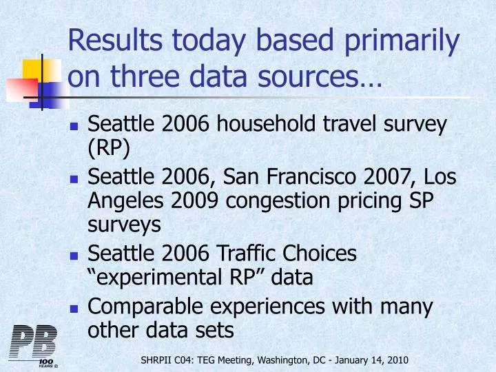
Results today based primarily on three data sources…. Seattle 2006 household travel survey (RP) Seattle 2006, San Francisco 2007, Los Angeles 2009 congestion pricing SP surveys Seattle 2006 Traffic Choices “experimental RP” data Comparable experiences with many other data sets.

E N D
Results today based primarily on three data sources… • Seattle 2006 household travel survey (RP) • Seattle 2006, San Francisco 2007, Los Angeles 2009 congestion pricing SP surveys • Seattle 2006 Traffic Choices “experimental RP” data • Comparable experiences with many other data sets SHRPII C04: TEG Meeting, Washington, DC - January 14, 2010
Seattle region (PSRC) RP data • 2006 household travel survey • Used 2-day place-based diary • 4700 HH, 90,000 trips • HW network times for SOV and HOV • 5 periods in the day (AM,MD,PM,EV,NT) • 17 periods in the day (mostly 1-hr long) • Separate skims of time on highly congested links SHRPII C04: TEG Meeting, Washington, DC - January 14, 2010
Models estimated on Seattle RP • Time of day choice (1 hour periods) • Mode choice (6 modes) • Joint time of day & mode choice • Two purpose groups: HBW, HBO • Two decision levels: trip-based, tour-based SHRPII C04: TEG Meeting, Washington, DC - January 14, 2010
General RP analysis approach • Time and cost only • Test specification of time variables • Add cost segmentation (income, occ.) • Add time segmentation • Add other explanatory variables SHRPII C04: TEG Meeting, Washington, DC - January 14, 2010
Findings- basic TOD tests • Based on time coefficient(s) only- No cost difference across TOD alternatives • Using departure time from home works better than using arrival time at work • Using arrival time back home works better than departure time from work • Using a restricted set of alternatives (6-8 hours) works better than all hours of day SHRPII C04: TEG Meeting, Washington, DC - January 14, 2010
Findings- basic TOD tests (2) • Variable of extra time on very congested links is highly correlated with travel time. Works best as a shift variable related to extra time in the worst hour (peak of the peak) • Similar findings from Sacramento data • May be proxy effect for variability SHRPII C04: TEG Meeting, Washington, DC - January 14, 2010
Mode choice nesting structure SHRPII C04: TEG Meeting, Washington, DC - January 14, 2010
Joint mode/TOD nesting structure (trip-based) • Tested seven different structures • HBW • Bottom level- nesting of one hour periods into broader time of day periods • Middle level – nesting of modes into groups • Top level – joint decision across mode groups and TOD groups (logsum close to 1.0) • HBO • Bottom level – nesting of modes into groups • Mode groups nested under one hour periods SHRPII C04: TEG Meeting, Washington, DC - January 14, 2010
Income and car occupancy included several ways… • Mode-specific dummy variables • Modifiers to cost effect • Modifiers to travel time effect • Time of day shift variables • Correlations between variables can cause instability SHRPII C04: TEG Meeting, Washington, DC - January 14, 2010
HBW- Imputed VOT by income and occupancy SHRPII C04: TEG Meeting, Washington, DC - January 14, 2010
HBW joint mode and TOD- tour-based • 8 departure hours from home x 7 arrival hours at home x 6 modes = 336 alternatives • Same mode nesting structure • No conclusive results yet on TOD nesting SHRPII C04: TEG Meeting, Washington, DC - January 14, 2010
RP analysis- tasks remaining • Add travel time variability measures for Seattle data • Add more “time pressure” variables to tour-based models – demonstrate value of activity-scheduling approach to influence value of travel time • Test transferability of models to Bay Area (BATS 2000) RP data SHRPII C04: TEG Meeting, Washington, DC - January 14, 2010
SP data analysis • Three main data sets… • Seattle : General toll scenarios: Free vs. tolled routes, Peak vs. off-peak • San Francisco: Downtown cordon pricing: Before, during or after peak, or transit • Los Angeles: HOT/Express lane scenarios: Free vs. tolled routes; before during or after peak, or transit (express bus via HOT lane) SHRPII C04: TEG Meeting, Washington, DC - January 14, 2010
SP analysis approach • Same general approach as for RP, but.. • More restricted… which alternatives and variables to include is largely pre-defined by the survey experiment • Tests mainly on segmentation and covariates • Allows “dynamic” analyses, such as departure time switching SHRPII C04: TEG Meeting, Washington, DC - January 14, 2010
Nesting for Seattle SP data SHRPII C04: TEG Meeting, Washington, DC - January 14, 2010
Nesting for San Francisco SP SHRPII C04: TEG Meeting, Washington, DC - January 14, 2010
Nesting for Los Angeles SP SHRPII C04: TEG Meeting, Washington, DC - January 14, 2010
Occupancy results-SP • In-vehicle time coefficient for HOV relative to SOV Work Non-work Seattle 1.03 1.39 San Francisco 1.12 1.90 Los Angeles 1.28 1.34 • No consistent effects on cost (?!) • SP responses may not reflect values of other vehicle occupants SHRPII C04: TEG Meeting, Washington, DC - January 14, 2010
Reliability results- SP • Seattle – each additional percent chance of a 15+ minute delay is equivalent to about 0.4 minutes travel time, for both work and non-work • San Francisco – each minute of extra delay at 10% probability is equivalent to about 0.15 minutes of travel time for work, and 0.5 minutes for non-work. Not as statistically significant as Seattle results. SHRPII C04: TEG Meeting, Washington, DC - January 14, 2010
SP analysis remaining • Very little – possible refinements to previous models • Compare to results of other SP-based studies SHRPII C04: TEG Meeting, Washington, DC - January 14, 2010
Seattle Traffic Choices data • “Experimental RP” – respondents given an amount of money and then charged by the mile for using main roads • Price varied by time of day/week and facility type • 500 vehicles with GPS units, experiment lasted more than a year >>> 750,000 trips • Some data collected during no-toll period SHRPII C04: TEG Meeting, Washington, DC - January 14, 2010
Traffic Choices analysis approach • Determine PSRC TAZ’s for trip ends • Skim best freeway and non-freeway paths for various times of day and attach to trip records • Analyze toll links actually used to determine the type of path chosen • Analyze toll distance and amount actually paid to confirm path choice • Estimate joint time of day / path type models, separately for HBW and HBO trips SHRPII C04: TEG Meeting, Washington, DC - January 14, 2010
Initial results • Based on very many observations • Toll variable very insignificant – high correlations between toll & travel time • Toll/distance or log(toll) gave better results • Nesting of route type under TOD – stronger for non-work than for work • Freeway route type constant increases with the fraction of path distance on freeway SHRPII C04: TEG Meeting, Washington, DC - January 14, 2010
Initial results (partial) HBW SHRPII C04: TEG Meeting, Washington, DC - January 14, 2010
Initial results (partial) HBO SHRPII C04: TEG Meeting, Washington, DC - January 14, 2010
Traffic Choice travel time reliability measures • Analyze all GPS travel times between pairs of network nodes • Determine mean, st.dev., 80th and 90th % time for each node pair/hour period • Aggregate node pairs into TAZ pairs and calculated weighted average of mean, st.dev., 80th and 90th % time • For each path type, apply st.dev./mean ratio to the network-based times SHRPII C04: TEG Meeting, Washington, DC - January 14, 2010
Results using reliability • Standard deviation of travel time negative and significant for HBW – similar to coefficient for travel time • But… wrong sign for HBO trips. • St.deviation per mile gave similar results • Toll coefficient now negative (included observations from post-tolling period) • Imputed VOT quite low ($5/hr) • Based on relatively few observations SHRPII C04: TEG Meeting, Washington, DC - January 14, 2010
Additional results HBW SHRPII C04: TEG Meeting, Washington, DC - January 14, 2010
Additional results HBO SHRPII C04: TEG Meeting, Washington, DC - January 14, 2010
Traffic Choices analysis remaining • Try to extend reliability measures to more node pairs and zone pairs… • Use a lower threshold of number of observations needed • Use only for periods with the most demand (or aggregate across other periods) • Use observed pairs to estimate synthesis equation • Match in household variables (income) SHRPII C04: TEG Meeting, Washington, DC - January 14, 2010
Summary comparison – absolute values of beta(time) SHRPII C04: TEG Meeting, Washington, DC - January 14, 2010
Conclusions (1) • Consistent willingness to pay for travel time savings across RP and SP data sets and types of models, but… • With important systematic differences by travel purpose, income and car occupancy SHRPII C04: TEG Meeting, Washington, DC - January 14, 2010
Conclusions (2) • For meaningful analysis of congestion pricing, time of day choice models are essential • Ideally, such models take advantage of data on current departure time or preferred departure or arrival time > time of day shift models SHRPII C04: TEG Meeting, Washington, DC - January 14, 2010
Conclusions (3) • Consistent evidence about hierarchy of types of travel decisions across RP & SP data sets… • Path type choice (toll/non-toll) is at the lowest level,conditional on other choices • For commuting, similar time periods nested underneath mode choice, but broader time of day periods generally above mode choice (similar to Dutch results) SHRPII C04: TEG Meeting, Washington, DC - January 14, 2010
Conclusions (4) • The effect of travel time variability is important, above and beyond the mean travel time • For OD-level analysis, std. deviation works better than 80th or 90th pctile, particularly when divided by distance • For application, simulation approaches best in the longer term (L04), but other approaches (link-based measures or synthesized OD measures) may be more feasible in the shorter term SHRPII C04: TEG Meeting, Washington, DC - January 14, 2010