Download
1 / 42
600 likes | 1.12k Views
Soil physics. Magnus Persson. 2·r. R. p-2q. 2·R·cos q. q. P 1. z. P 2. Surface tension. Due to surface tension water can be held at negative pressure in capillary tubes. (P 1 <P 2 = P atm ) The smaller the diameter of the tube, the higher capillary rise.

E N D
Soil physics Magnus Persson
2·r R p-2q 2·R·cos q q P1 z P2 Surface tension Due to surface tension water can be held at negative pressure in capillary tubes. (P1<P2 = Patm) The smaller the diameter of the tube, the higher capillary rise. An useful analogy is that the soil can be considered to act like a bundle of cappilary tubes with different diameters (representing the range of pore sizes)
pF curve The soil moisture potential, or soil water suction, is sometimes given in pF = log(-pressure in cm H2O). The water retention curve, soil moisture characteristic, or pF curve, is the relationship between the water content, θ, and the soil water potential, ψ. This curve is characteristic for different types of soil (1 bar = 100 kPa = 1000 cm H2O)
Soil water potential • The total potential consists of the moisture potential (synonyms; pore water tension, soil water suction) and the elevation potential, z. • Normally the groundwater surface is used as a reference level (z = 0)
Water movement Water movement is driven by total potential gradients
q z dz Theory of one-dimensional unsaturated water flow Using continuity (inflow – outflow = change in storage over time) we get (1) where is the volumetric water content andt is time.
Theory of one-dimensional unsaturated water flow The Darcy law gives us that (2) where H is the total potential. The total potential consists of the moisture potential (synonyms; pore water tension, soil water suction) and the elevation potential, z. Thus (3) Combining (1) and (3) we get (4) This is called the Richard equation. Remember that and K both are functions of .
Theory of one-dimensional unsaturated water flow There is a soil specific relationship between soil water content and moisture potential and hydraulic conductivity. The soil moisture potential, or soil water suction, is sometimes given in pF = log(-pressure in cm H2O)
Theory of one-dimensional unsaturated water flow Several models exists for these relationships, today, the most commonly used were presented by van Genuchten (1980). (5) (6) where n, m, and are soil specific parameters, r and s are residual and saturated water content, respectively. The term Ks is the saturated hydraulic conductivity. The parameter r is usually assumed to be equal to the water content at a suitable low pressure head, e.g., -150 m H2O, i.e., the wilting point (pF 4.2).
Infiltration • A special case of one-dimensional unsaturated water flow is infiltration • Infiltration is of interest in hydrology (rainfall-runoff relationship) and Agriculture (irrigation). • Infiltration parameters for different soil types are determined in infiltration experiments
Infiltration Two cases of wetting fronts, in the first, the infiltration rate i is lower than the saturated hydraulic conductivity Ks
Infiltration models • Green-Ampt where I is the cumulative infiltration, Lfis the wetting front depth, ΔΨ is the change in potential between the soil surface and the wetting front (tabled values exists, see next slide) It can be assumed that I = Lf (θt - θi)
Infiltration models Soil parameters (Green-Ampt)
Infiltration models Horton where fo = infiltration capacity in dry soil (mm/h) fc = = infiltration capacity in wet soil (mm/h) k = time factor (h-1)
Solute transport Solute transport processes in unsaturated soil advection
Solute transport The dispersion coefficient includes effect of both molecular diffusion and mechanical dispersion. Dispersivity = Dispersion coefficient/velocity
Solute transport The solute transport in the saturated and unsaturated zones can be modeled using the advection-dispersion equation (ADE) where D is the dispersion coefficient, R is the retardation coefficient (sorption), and vz is the (vertical) water velocity. In the groundwater, the water velocity is calculated by the Darcy law, in the unsaturated zone the water velocity is calculated using Richards’s equation. Can also include source/sink terms, (chemical reactions, biodegredation)
Solute transport Analythical solution of the CDE for a pulse input and constant v and D where M is the applied mass and A is the cross sectional area.
Different concepts In the ADE concept described above, transport is governed by advection and dispersion. A different approach is the stochastic-advective concept. In this concept, solutes are transported in isolated stream tubes by advection only. The velocity distribution of the stream tubes can be described by a stochastic probability density function (pdf).
Different concepts Solute transport concepts Convective-dispersive Stochastic-convective
Stochastic convective approach Assuming that the solute is spread instantaneously at z=0 and that the average solute transport velocity is constant, the Crt*(z,t) can be described by where l is the mean of the lognormal pdf and l2 is the corresponding variance for the reference depth l.
Stochastic convective approach The l parameter of the CLT model is related to the variability of the velocity distribution. This can be considered to be a soil specific parameter, however, it will also be slightly dependent on the magnitude of the soil water flux. The where l can be used to calculate the average pore water velocity v using
ALT vs. ADE Both models calibrated to measurements at 0.235 m depth.
ALT vs. ADE Predicted BTCs at 0.6 m depth
Questions Discuss one of these questions in small groups and present the answer to the others
Soil properties may change dramatically over short distances. Water will not flow uniformly in the soil profile, but may flow in so called macropores, i.e., along roots, desiccation cracks or worm holes. This is called preferential flow. Macropore flow is often triggered at a specific water content and may lead to that large amounts of solutes are transported directly to the groundwater. Spatial variability
Macropores Macropores (desiccation cracks) in a clay soil in Egypt
Water drop penetration test • Water repellency can be determined with the water drop penetration test (WDPT) • The procedure is as follows: • 5 – 30 g sample of dry soil is put on a horizontal surface. • The samples are leveled and a small 2-3 mm drop of water is added to the surface of the soil. • On non-wetting soils the water will form a ball and stay on the surface for a time. • Record the time for the drop to infiltrate. • The test should be repeated at least three times and the average time should be recorded.
How to account for variability • Dual porosity models (e.g., MACRO) • Stream tube models • Stochastic models • Fractal models
Fractal models • One model capable of generating fractal clusters i the DLA model. Diffusion limited aggregation conceptually describes the growth of crystals. • This model has been successfully applied to solute transport
Literature and links • http://www.ars.usda.gov/Services/docs.htm?docid=15992 (models for download) • http://wwwbrr.cr.usgs.gov/projects/GW_Unsat/Unsat_Zone_Book/index.html (online textbook) • Persson and Berndtsson, 1999. Water application frequency effects on steady-state solute transport parameters J. Hydrol. 225:140-154 • http://www.pc-progress.cz/Default.htm (hydrus 1D code) • http://bgf.mv.slu.se/ShowPage.cfm?OrgenhetSida_ID=5658 (MACRO model)