Download
1 / 52
520 likes | 625 Views
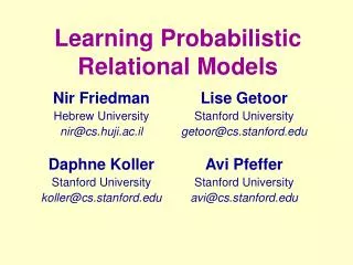
Learning Probabilistic Relational Models. Lise Getoor 1 , Nir Friedman 2 , Daphne Koller 1 , and Avi Pfeffer 3 1 Stanford University, 2 Hebrew University, 3 Harvard University. Overview. Motivation Definitions and semantics of probabilistic relational models (PRMs) Learning PRMs from data

E N D
Learning Probabilistic Relational Models Lise Getoor1, Nir Friedman2, Daphne Koller1, and Avi Pfeffer3 1Stanford University, 2Hebrew University, 3Harvard University
Overview • Motivation • Definitions and semantics of probabilistic relational models (PRMs) • Learning PRMs from data • Parameter estimation • Structure learning • Experimental results
Motivation • Most real-world data are stored in relational DBMS • Few learning algorithms are capable of handling data in its relational form; thus we have to resort to “flattening” the data in order to do analysis • As a result, we lose relational information which might be crucial to understanding the data
Related Work • Most inductive logic programming (ILP) approaches are deterministic classification approaches, i.e. they do not attempt to model a probability distribution but rather learn a set of rules for classifying when a particular predicate holds • Recent developments in ILP related to PRMs: • Stochastic logic programs (SLPs) [Muggleton, 1996 and Cussens, 1999] • Bayesian logic programs (BLPs) [Kersting et al., 2000]
What are PRMs? • The starting point of this work is the structured representation of probabilistic models of Bayesian networks (BNs). BNs for a given domain involves a pre-specified set of attributes whose relationship to each other is fixed in advance • PRMs conceptually extend BNs to allow the specification of a probability model for classes of objects rather than a fixed set of simple attributes • PRMs also allow properties of an entity to depend probabilistically on properties of other related entities
Mapping PRMs from Relational Models • The representation of PRMs is a direct mapping from that of relational databases • A relational model consists of a set of classes X1,…,Xn and a set of relations R1,…,Rm,where each relation Ri is typed • Each class or entity type (corresponding to a single relational table) is associated with a set of attributesA(Xi) and a set of reference slots R (X)
PRM Semantics • Reference slots correspond to attributes that are foreign keys (key attributes of another table) • X.ρ, is used to denote reference slot ρ of X. Each reference slot ρ is typed according to the relation that it references
Primary keys are indicated by a blue rectangle Indicates many-to-many relationship Indicates one-to-many relationship Underlined attributes are reference slots of the class Dashed lines indicate the types of objects referenced University Domain Example - Relational Schema M 1 Professor Student Name Name Popularity Intelligence Ranking Teaching-Ability 1 Registration Course RegID Name Course Instructor M M Student Rating M Grade Difficulty Satisfaction
PRM Semantics Continued • Each attribute AjA(Xi) takes on values in some fixed domain of possible values denoted V(Aj). We assume that value spaces are finite • Attribute A of class X is denoted X.A • For example, the Student class has an Intelligence attribute and the value space or domain for Student.Intelligence might be {high, low}
PRM Semantics Continued • An instanceI of a schema specifies a set of objects x, partitioned into classes; such that there is a value for each attribute x.A and a value for each reference slot x.ρ • A(x) is used as a shorthand for A(X), where x is of class X. For each object x in the instance and each of its attributes A, we use Ix.A to denote the value of x.A in I
Professor Name Prof. Gump Popularity high Teaching-Ability medium Student Name Jane Doe Intelligence high Ranking average Student Name Jane Doe Intelligence high Ranking average Registration RegID #5639 Grade A Satisfaction 3 Course Name Phil101 Difficulty low Rating high Registration RegID #5639 Grade A Satisfaction 3 Course Name Phil101 Difficulty low Rating high Registration RegID #5639 Grade A Satisfaction 3 University Domain Example – An Instance of the Schema One professor is the instructor for both courses Jane Doe is registered for only one course, Phil101, while the other student is registered for both courses
University Domain Example – Another Instance of the Schema Professor Name Prof. Vincent Popularity high Teaching-Ability high Student Name Jane Doe Intelligence high Ranking average Professor Name Prof. Gump Popularity high Teaching-Ability medium Student Name Jane Doe Intelligence high Ranking average Student Name John Doe Intelligence high Ranking average There are two professors instructing a course Registration RegID #5639 Grade A Satisfaction 3 Registration RegID #5639 Grade A Satisfaction 3 There are three students in the Phil201 course Course Name Phil201 Difficulty low Rating high Registration RegID #5723 Grade A Satisfaction 3
PRM Semantics Continued • Some attributes, such as name or social security number, are fully determined. Such attributes are labeled as fixed. Assume that they are known in any instantiation of the schema • The other attributes are called probabilistic
Probabilistic attributes are shown in italic Fixed attributes are shown in regular font Probabilistic attributes are shown in italic Fixed attributes are shown in regular font University Domain Example - Relational Schema M 1 Professor Student Name Name Popularity Intelligence Ranking Teaching-Ability 1 Registration Course RegID Name Course Instructor M M Student Rating M Grade Difficulty Satisfaction
PRM Semantics Continued • A skeleton structure σof a relational schema is a partial specification of an instance of the schema. It specifies the set of objects Oσ(Xi) for each class, the values of the fixed attributes of these objects, and the relations that hold between the objects • The values of probabilistic attributes are left unspecified • A completion I of the skeleton structure σ extends the skeleton by also specifying the values of the probabilistic attributes
Professor Name Prof. Gump Popularity ??? Teaching-Ability ??? Student Name Jane Doe Intelligence high Ranking average Student Name Jane Doe Intelligence ??? Ranking ??? Registration RegID #5639 Grade A Satisfaction 3 Course Name Phil101 Difficulty low Rating high Registration RegID #5639 Grade A Satisfaction 3 Course Name Phil101 Difficulty ??? Rating ??? Registration RegID #5639 Grade ??? Satisfaction ??? University Domain Example – Relational Skeleton
Professor Name Prof. Gump Popularity high Teaching-Ability medium Student Name Jane Doe Intelligence high Ranking average Student Name Jane Doe Intelligence high Ranking average Registration Name #5639 Grade A Satisfaction 3 Course Name Phil101 Difficulty low Rating high Registration Name #5639 Grade A Satisfaction 3 Course Name Phil101 Difficulty low Rating high Registration Name #5639 Grade A Satisfaction 3 University Domain Example – The Completion Instance I
University Domain Example – Another Relational Skeleton Professor Name Prof. Vincent Popularity ??? Teaching-Ability ??? Student Name Jane Doe Intelligence high Ranking average Professor Name Prof. Gump Popularity high Teaching-Ability ??? Student Name Jane Doe Intelligence high Ranking average Student Name John Doe Intelligence ??? Ranking ??? Registration RegID #5639 Grade A Satisfaction 3 Registration RegID #5639 Grade A Satisfaction 3 PRMs allow multiple possible skeletons Course Name Phil201 Difficulty ??? Rating ??? Registration RegID #5723 Grade ??? Satisfaction ???
University Domain Example – The Completion Instance I Professor Name Prof. Vincent Popularity high Teaching-Ability high Student Name Jane Doe Intelligence high Ranking average Professor Name Prof. Gump Popularity high Teaching-Ability medium Student Name Jane Doe Intelligence high Ranking average Student Name John Doe Intelligence high Ranking average Registration RegID #5639 Grade A Satisfaction 3 Registration RegID #5639 Grade A Satisfaction 3 PRMs also allow multiple possible instances and values Course Name Phil201 Difficulty low Rating high Registration RegID #5723 Grade A Satisfaction 3
More PRM Semantics • For each reference slot ρ, we define an inverse slot, ρ-1, which is the inverse function of ρ • For example, we can define an inverse slot for the Student slot of Registration and call it Registered-In. Since the original relation is a one-to-many relation, it returns a set of Registration objects • A final definition is the notion of a slot chain τ=ρ1..ρm, which is a sequence of reference slots that defines functions from objects to other objects to which they are indirectly related. For example, Student.Registered-In.Course.Instructor can be used to denote a student’s set of instructors
Definition of PRMs • The probabilistic model consists of two components: the qualitative dependency structure, S, and the parameters associated with it, θS • The dependency structure is defined by associating with each attribute X.A a set of parents Pa(X.A); parents are attributes that are “direct influences” on X.A. This dependency holds for any object of class X
Definition of PRMs Cont’d • The attribute X.A can depend on another probabilistic attribute B of X. This dependence induces a corresponding dependency for individual objects • The attribute X.A can also depend on attributes of related objects X.τ.B, where τ is a slot chain • For example, given any Registration object r and the corresponding Professor object p for that instance, r.Satisfaction will depend probabilistically on r.Grade as well as p.Teaching-Ability
Edges correspond to probabilistic dependency for objects in that class M Professor Student Teaching-Ability Intelligence Ranking Popularity M 1 1 Course M M Rating Registration Satisfaction Edges from one class to another are routed through slot-chains Difficulty Grade PRM Dependency Structure for the University Domain
Dependency Structure in PRMs • As mentioned earlier, x.τ represents the set of objects that are τ-relatives of x. Except in cases where the slot chain is guaranteed to be single-valued, we must specify the probabilistic dependence of x.A on the multiset {y.B:y x.τ} • The notion of aggregation from database theory gives us the tool to address this issue; i.e., x.a will depend probabilistically on some aggregate property of this multiset
Aggregation in PRMs • Examples of aggregation are: the mode of the set (most frequently occurring value); mean value of the set (if values are numerical); median, maximum, or minimum (if values are ordered); cardinality of the set; etc • An aggregate essentially takes a multiset of values of some ground type and returns a summary of it • The type of the aggregate can be the same as that of its arguments, or any type returned by an aggregate. X.A can have γ(X.τ.B) as a parent; the semantics is that for any x X, x.a will depend on the value of γ(x.τ.b), V(γ(x.τ.b))
Student Intelligence Ranking Course Rating Difficulty PRM Dependency Structure M Professor A student may take multiple courses Teaching-Ability Popularity M 1 1 M M Registration AVG Satisfaction The student’s ranking depends on the average of his grades AVG A course rating depends on the average satisfaction of students in the course Grade
Parameters of PRMs • A PRM contains a conditional probability distribution (CPD) P(X.A|Pa(X.A)) for each attribute X.A of each class • More precisely, let U be the set of parents of X.A. For each tuple of values uV(U), the CPD specifies a distribution P(X.A|u) over V(X.A). The parameters in all of these CPDs comprise θS
M Professor Student Teaching-Ability Intelligence M 1 Ranking Popularity 1 M M Registration Course Satisfaction Rating Grade Difficulty CPDs in PRMs AVG AVG D.I A B C h,h 0.5 0.4 0.1 h,l 0.1 0.5 0.4 l,h 0.8 0.1 0.1 l,l 0.3 0.6 0.1 avg l m h A 0.1 0.2 0.7 B 0.2 0.4 0.4 C 0.6 0.3 0.1
Parameters of PRMs Continued • Given a skeleton structure for our schema, we want to use these local probability models to define a probability distribution over all completions of the skeleton • Note that the objects and relations between objects in a skeleton are always specified by σ, hence we are disallowing uncertainty over the relational structure of the model
Parameters of PRMs Continued • To define a coherent probabilistic model, we must ensure that our probabilistic dependencies are acyclic, so that a random variable does not depend, directly or indirectly, on its own value • A dependency structure S is acyclic relative to a skeleton σ if the directed graph over all the parents of the variables x.A is acyclic • If S is acyclic relative to σ, then the following defines a distribution over completions I of σ: P(I|σ,S,θS) =
Class Dependency Graph for the University Domain Course.Difficulty Student.Intelligence Professor.Teaching-Ability Registration.Grade Registration.Satisfaction Student.Ranking Professor.Popularity Course.Rating
Ensuring Acyclic Dependencies • In general, however, a cycle in the class dependency graph does not imply that all skeletons induce cyclic dependencies • A model may appear to be cyclic at the class level, however, this cyclicity is always resolved at the level of individual objects • The ability to guarantee that the cyclicity is resolved relies on some prior knowledge about the domain. The user can specify that certain slots are guaranteed acyclic
Person Person BloodType BloodType Person P-chromosome P-chromosome P-chromosome M-chromosome M-chromosome M-chromosome BloodType Contaminated Result BloodTest PRM for the Genetics Domain (Father) (Mother)
Dependency Graph for Genetics Domain Person.M-chromosome Person.P-chromosome Person.BloodType Dashed edges correspond to “guaranteed acyclic” dependencies BloodTest.Contaminated BloodTest.Result
Learning PRMs: Parameter Estimation • Assume that the qualitative dependency structure S of the PRM is known • The parameters are estimated using the likelihood function which gives an estimate of the probability of the data given the model • The likelihood function used is the same as that for Bayesian network parameter estimation. The only difference is that parameters for different nodes in the network – those corresponding to the x.A for different objects x from the same class – are forced to be identical
Learning PRMs: Parameter Estimation • Our goal is to find the parameter setting θS that maximizes the likelihood L(θS| I,σ,S) for a given I, σ and S: L(θS|I,σ,S) = P(I|σ,S,θS). Working with the logarithm of this function: l(θS|I,σ,S) = log P(I|σ,S,θS) = • This estimation is simplified by the decomposition of log-likelihood function into a summation of terms corresponding to the various attributes of the different classes. Each of the terms in the square brackets can be maximized independently of the rest • Parameter priors can also be incorporated
Learning PRMs: Structure Learning • We now move to the more challenging problem of learning a dependency structure automatically • There are three important issues that need to be addressed: hypothesis space, scoring function, and search algorithm • Our hypothesis specifies a set of parents for each attribute X.A. Note that this hypothesis space is infinite. Our hypothesis space is restricted by ensuring that the structure we are learning will generate a consistent probability model for any skeleton we are likely to see
Learning PRMs: Structure Learning Continued • The second key component is the ability to evaluate different structures in order to pick one that fits the data well. Bayesian model selection methods were adapted • Bayesian model selection utilizes a probabilistic scoring function. It ascribes a prior probability distribution over any aspect of the model about which we are uncertain • The Bayesian score of a structure S is defined as the posterior probability of the structure given the data I
Learning PRMs: Structure Learning Continued • Using Bayes rule: P(S|I,σ) P(I|S,σ) P(S|σ) • It turns out that marginal likelihood is a crucial component, which has the effect of penalizing models with a large number of parameters. Thus this score automatically balances the complexity of the structure with its fit to the data • Now we need only provide an algorithm for finding a high-scoring hypotheses in our space
Learning PRMs: Structure Learning Continued • The simplest heuristic search algorithm is greedy hill-climbing search, using the scoring function as a metric. Maintain the current candidate structure and iteratively improve it • Local maxima can be dealt with using random restarts, i.e., when a local maximum is reached, we take a number of random steps, and then continue the greedy hill-climbing process
Learning PRMs: Structure Learning Continued • The problems with this simple approach is that there are infinitely many possible structures, and it is very costly in computational operations • A heuristic search algorithm addresses these issues. At a high level, the algorithm proceeds in phases
Learning PRMs: Structure Learning Continued • At each phase k, we have a set of potential parents Potk(X.A) for each attribute X.A • Then apply a standard structure search restricted to the space of structures in which the parents of each X.A are in Potk(X.A). The phased search is structured so that it first explores dependencies within objects, then between objects that are directly related, then between objects that are two links apart, etc
Learning PRMs: Structure Learning Continued • One advantage of this approach is that it gradually explores larger and larger fragments of the infinitely large space, giving priority to dependencies between objects that are more closely related • The second advantage is that we can precompute the database view corresponding to X.A, Potk(X.A); most of the expensive computations – the joins and aggregation required in the definition of the parents – are precomputed in these views
Experimental Results • The learning algorithm was tested on one synthetic dataset and two real ones • Genetics domain – a artificial genetic database similar to the example mentioned earlier was used to test the learning algorithm • Training sets of size 200 to 800, with 10 training sets of each size were used. An independent test database of size 10,000 was also generated • A dataset size of n consists of a family tree containing n people, with an average of 0.6 blood tests per person
Experimental Results Continued • Tuberculosis patient domain – drawn from a database of epidemiological data for 1300 patients from the SF tuberculosis (TB) clinic, and their 2300 contacts • Relational dependencies, along with other interesting dependencies, were discovered: there is a dependence between the patient’s HIV result and whether he transmits the disease to a contact; there is a correlation between the ethnicity of the patient and the number of patients infected by the strain
Experimental Results Continued • Company domain – a dataset of company and company officers obtained from Security and Exchange Commission (SEC) data • The dataset includes information, gathered over a five year period, about companies, corporate officers in the companies, and the role that the person plays in the company • For testing, the following classes and table sizes were used: Company (20,000), Person (40,000), and Role (120,000)
Discussion • How do you determine the probability distribution when there is an unbound variable? • The literature assumes that domain values are finite. Can it handle continuous values?