Download
1 / 37
370 likes | 596 Views
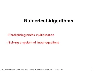
Numerical Algorithms. .Matrix Multiplication .Gaussian Elimination .Jacobi Iteration .Gauss-Seidel Relaxation. Numerical Algorithms. Matrix addition. Numerical Algorithms. Matrix Multiplication. Numerical Algorithms. Matrix-Vector Multiplication. Implementing Matrix Multiplication.

E N D
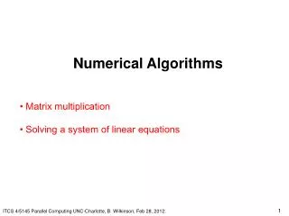
Numerical Algorithms .Matrix Multiplication .Gaussian Elimination .Jacobi Iteration .Gauss-Seidel Relaxation
Numerical Algorithms Matrix addition
Numerical Algorithms Matrix Multiplication
Numerical Algorithms Matrix-Vector Multiplication
Implementing Matrix Multiplication Sequential Code O(n3) for(i=0 ; i<n ; i++) for(j=0 ; j<n ; j++){ c[i][j] = 0; for(k=0 ; k<n ; k++) c[i][j] = c[i][j] + a[i][k] * b[k][j]; }
Implementing Matrix Multiplication Partitioning into Submatrices for(p=0 ; p<s ; p++) for(q=0 ; q<s ; q++){ Cp,q = 0; for(r=0 ; r<m ; r++) Cp,q = Cp,q + Ap,r * Br,q; }
Implementing Matrix Multiplication Analysis communication computation
Implementing Matrix Multiplication O(n2) with n2 processorsO(log n) with n3 processors
Implementing Matrix Multiplication submatrices s=n/m communication computation
Recursive Implementation mat_mult(App, Bpp, s) { if( s==1) C=A*B; else{ s = s/2; P0 = mat_mult(App, Bpp, s); P1 = mat_mult(Apq, Bqp, s); P2 = mat_mult(App, Bpq, s); P3 = mat_mult(Apq, Bqq, s); P4 = mat_mult(Aqp, Bpp, s); P5 = mat_mult(Aqq, Bqp, s); P6 = mat_mult(Aqp, Bpq, s); P7 = mat_mult(Aqq, Bqq, s); Cpp = P0 + P1; Cpq = P2 + P3; Cqp = P4 + P5; Cqq = P6 + P7; } return(C); }
Mesh Implementation Connon's Algorithm 1. initially processor Pij has element Aij and Bij 2. Elements are moved from their initial position to an "aligned" position. The complete ith row of A is shifted i places left and the complete jth column of B is shifted j places downward. this has the effect of placing the elements aij+1 and the element bi+jj in processor Pij, as illusrated in figure 10.10. These elements are pair of those required in the accumulation of cij 3. Each processor, P1j, multiplies its elements. 4. The ith row of A is shifted one place right, and the jth column of B is shifted one place downward. this has the effect of bringing together the adjacent elements of A and B, which will also be required in the accumulation, as illustrated in Figure 10.11. 5. Each processor, Pij, multiplies the elements brought to it and adds the result to the accumulation sum. 6. Step 4 and 5 are repeated until the final result is obtained
Mesh Implementation Analysis O(sm2) communication computation
Two dimensional pipeline--- Systolic array recv(&a, Pi,j-1); recv(&b, Pi-1,j); c=c+a*b; send(&a, Pi,j+1); send(&b, Pi+1,j);
Solving a System of Linear Equations Ax=b Dense matrix Sparse matrix
Solving a System of Linear Equations Gaussian Elimination
Solving a System of Linear Equations O(n3) for(i=0 ; i<n-1 ; i++) for(j=i+1 ; j<n ; j++){ m = a[j][i]/a[i][i]; for(k=i ; k<n ; k++) a[j][k] = a[j][k] - a[i][k] * m; b[j] = b[j] - b[i] * m;
Solving a System of Linear Equations communication O(n2)
Solving a System of Linear Equations computation
Solving a System of Linear Equations Pipeline configuration
Iterative Methods Jacobi Iteration
Iterative Methods Relationship with a General System of Linear Equations
Iterative Methods Gauss-Seidel Relaxation
Iterative Methods Red-Black Ordering
Iterative Methods forall(i=0 ; i<n ; i++) forall(j=1 ; j<n ; j++) if((i+j)%2 == 0) f[i][j] = 0.25*(f[i-1][j]+f[i][j-1]+f[i+1][j]+f[i][j+1]); forall(i=1 ; i<n ; i++) forall(j=1 ; j<n ; j++) if((i+j)%2 !=0 ) f[i][j] = 0.25*(f[i-1][j]+f[i][j-1]+f[i+1][j]+f[i][j+1]);
Iterative Methods High-Order Difference Methods
Iterative Methods Multigrid Method