Download

1 / 64
800 likes | 1.53k Views
Repeated Measure Design of ANOVA. AMS 572 Group 5. Outline. Jia Chen: Introduction of repeated measures ANOVA Chewei Lu: One-way repeated measures Wei Xi: Two-factor repeated measures Tomoaki Sakamoto : Three-factor repeated measures How-Chung Liu: Mixed models

E N D
Repeated Measure Design of ANOVA AMS 572 Group 5
Outline • Jia Chen: Introduction of repeated measures ANOVA • Chewei Lu: One-way repeated measures • Wei Xi: Two-factor repeated measures • Tomoaki Sakamoto : Three-factor repeated measures • How-Chung Liu: Mixed models • Margaret Brown: Comparison • Xiao Liu: Conclusion
What is it ? Definition: - It is a technique used to test the equality of means.
When To Use It? • It is used when all members of a random sample are measured under a number of different conditions. • As the sample is exposed to each condition in turn, the measurement of dependent variable is repeated.
Introduction of One-Way Repeated Measures ANOVA Che-Wei, Lu Professor:Wei Zhu
One-Way Repeated Measures ANOVA • Definition A one-way repeated measures ANOVA instead of having one score per subject, experiments are frequently conducted in which multiple score are gathered for each case. • Concept of Repeated Measures ANOVA • One factor with at least two levels, levels are dependent. • Dependent means that they share variability in some way. • The Repeated Measures ANOVA is extended from standard ANOVA.
One-Way Repeated Measures ANOVA • When to Use • Measuring performance on the same variable over time • for example looking at changes in performance during training or before and after a specific treatment • The same subject is measured multiple times under different conditions • for example performance when taking Drug A and performance when taking Drug B • The same subjects provide measures/ratings on different characteristics • for example the desirability of red cars, green cars and blue cars • Note how we could do some RM as regular between subjects designs • For example, Randomly assign to drug A or B
One-Way Repeated Measures ANOVA • Source of Variance in Repeated Measures ANOVA • SStotal • Deviation of each individual score from the grand mean • SSb/t subjects • Deviation of subjects' individual means (across treatments) from the grand mean. • In the RM setting, this is largely uninteresting, as we can pretty much assume that ‘subjects differ’ • SSw/in subjects: How Ss vary about their own mean, breaks down into: • SStreatment • As in between subjects ANOVA, is the comparison of treatment means to each other (by examining their deviations from the grand mean) • However this is now a partition of the within subjects variation • SSerror • Variability of individuals’ scores about their treatment mean
One-Way Repeated Measures ANOVA • Partition of Sum of Square Repeated Measures ANOVA Standard ANOVA
One-Way Repeated Measures ANOVA • Standard ANOVA Table • Repeated Measures ANOVA Table
One-Way Repeated Measures ANOVA • Example: Researchers want to test a new anti-anxiety medication. They measure the anxiety of 7 participants three times: once before taking the medication, once one week after taking the medication, and once two weeks after taking medication. Anxiety is rated on a scale of 1-10,with 10 being ”high anxiety” and 1 being “low anxiety”. Are there any difference between the three condition using significant level
One-Way Repeated Measures ANOVA • Define Null and Alternative Hypotheses
One-Way Repeated Measures ANOVA • Define Degrees of Freedom N=21 s=7 -=18-6=12
One-Way Repeated Measures ANOVA • Analysis of Variance
One-Way Repeated Measures ANOVA • Analysis of Variance(ANOVA Table) Error=within-Subjects=10.29-7.62=2.67 Total=Beteen+Within=98.67+10.29=108.96 • Test Statistic: 244.27
One-Way Repeated Measures ANOVA • Critical Region Now, the
One-Way Repeated Measures ANOVA DATA REPEAT; INPUT SUBJ BEFORE WEEK1 WEEK2; DATALINES; 1 9 7 4 2 8 6 3 3 7 6 2 4 8 7 3 5 8 8 4 6 9 7 3 7 8 6 2 ; PROCANOVA DATA=REPEAT; TITLE "One-Way ANOVA using the repeated Statment"; MODEL BEFORE WEEK1 WEEK2= / NOUNI; REPEATED TIME 3 (123); RUN; The Before, Week1, and Week2 are the time level at each participants. • SAS Code The NOUNI(no univariate) is a request not to conduct a separate analysis for each of the three times variables. In here, we don’t have CLASS statement because our data set does not have an independent variable This indicates the labels we want to printed for each level of times
One-Way Repeated Measures ANOVA • SAS Result
Example • The shape variable is the repeated variable. This produces an ANOVA with one between-subjects factor. If you were to examine the expected mean squares for this setup, you would find that the appropriate error term for the test of calib is subject|calib. The appropriate error term for shape and shape#calib is shape#subject|calib (which is the residual error since we do not include the term in the model).
SAS Code Data Q1; set pre.Q1; run; procanova data=Q1; title' Two-way Anova with a Repeated Measure on One Factor'; class calib; model shape_1 shape_2 shape_3 shape_4 = calib/nouni; repeated shape 4; means calib; run;
Analysis of SAS Output At α=0.05,we reject the hypothesis and conclude that there is shape Effect At α=0.05,we cannotreject the hypothesis and conclude that there is no shape*calib Effect
Tests of Hypotheses for Between Subjects Effects Univariate Tests of Hypotheses for Within Subject Effects
Example • Three subjects, each with nine accuracy scores on all combinations of the three different dials and three different periods. With subject a random factor and both dial and period fixed factors, the appropriate error term for the test of dial is the dial#subject interaction. Likewise, period#subject is the correct error term for period, and period#dial#subject (which we will drop so that it becomes residual error) is the appropriate error term for period#dial.
SAS Code • Data Q2; • Input Mins1-Mins9; • Datalines; • 45 53 60 40 52 57 28 37 46 • 35 41 50 30 37 47 28 32 41 • 60 65 75 58 54 70 40 47 50 • ; • ODS RTF STYLE=BarrettsBlue; • Proc anova data=Q2; • Model Mins1-Mins9=/nouni; • Repeated period 3, dail 3/nom; • Run; • ods rtf close;
SAS Output Univariate Tests of Hypotheses for Within Subject Effects At α=0.05,we reject the hypothesis and conclude that there is period Effect At α=0.05,we reject the hypothesis and conclude that there is dail Effect At α=0.05,we cannot reject the hypothesis and conclude the there is no period*dail Effect
Three-factor Experiments with a repeated measure T. Sakamoto
Example of a marketing experiment • Case of this example • A company which produces some Liquid Crystal Display wants to examine the characteristics of its prototype products. • Experiment • The subjects who belong to a region X or Y see the Liquid Crystal Display A, B, or C. • Each type of LCD is seen twice; once in the light and the other in the dark. • The preferences of the LCD are measured by the subjects, on a scale from 1 to 5 (1= lowest, 5=highest).
Experimental Design and Data • Three factors • Type of LCD • Regions to which the specimens belong • In the light / In the dark • Repeted measure factor : In the light / In the dark
SAS PROGRAM • data lcd; • input subj type $ region $ light dark @@; • datalines; • 1 a 5 4 2 a 4 2 3 a 5 4 4 a 3 5 5 a 5 3 • 6 a 4 4 7 a 3 5 8 a 4 3 9 a 2 5 10 a 5 4 • 11 b 4 4 12 b 5 6 13 b 3 4 14 b 5 4 15 b 4 6 • 16 b 5 5 17 b 4 3 18 b 5 3 19 b 5 5 20 b 4 4 • 21 c 5 5 22 c 5 3 23 c 3 3 24 c 4 4 25 c 4 3 • 26 c 3 5 27 c 4 3 28 c 5 2 29 c 3 4 30 c 4 3 • ; • run; • proc anovadata=lcd; • title’Three-way ANOVA with a Repeated Measure'; • class type region; • model light dark = type | region /nouni; • repeated light_dark; • means type | region; • run;
OUTPUT(Part 3/4): 40/81
Mixed Effect Models How-Chang Liu
Mixed Models • When we have a model that contains random effect as well as fixed effect, then we are dealing with a mixed model. • From the above definition, we see that mixed models must contain at least two factors.One having fixed effect and one having random effect.
Why use mixed models? • When repeated measurements are made on the same statistical units, it would not be realistic to assume that these measurements are independent. • We can take this dependence into account by specifying covariance structures using a mixed model
Definition • A mixed model can be represented in matrix notation by: • is the vector of observations • is the vector of fixed effects • is the vector of random effects • is the vector of I.I.D. error terms • and are matrices relating and to
Assumptions • R and G are constants • We also assume that and are independent • We get V = ZGZ' + R, where V is the variance of y
How to estimate and ? If R and G are given: Using Henderson’s Mixed Model equation, we have: = So = And = )
What if G and R are unknown? • We know that both and are normally distributed, so the best approach is to use likelihood based methods • There are two methods used by SAS: • 1)Maximum likelihood (ML) • 2)Restricted/residual maximum likelihood (REML)
Example Below is a table of growth measurements for 11 girls and 16 boys at ages 8, 10, 12, 14: Person gender age8 age10 age12 age14 1 F 21.0 20.0 21.5 23.0 2 F 21.0 21.5 24.0 25.5 3 F 20.5 24.0 24.5 26.0 4 F 23.5 24.5 25.0 26.5 5 F 21.5 23.0 22.5 23.5 6 F 20.0 21.0 21.0 22.5 7 F 21.5 22.5 23.0 25.0 8 F 23.0 23.0 23.5 24.0 9 F 20.0 21.0 22.0 21.5 10 F 16.5 19.0 19.0 19.5 11 F 24.5 25.0 28.0 28.0 12M 26.0 25.0 29.0 31.0 13 M 21.5 22.5 23.0 26.5 14 M 23.0 22.5 24.0 27.5 Person gender age8 age10 age12 age14 15 M 25.5 27.5 26.5 27.0 16 M 20.0 23.5 22.5 26.0 17 M 24.5 25.5 27.0 28.5 18 M 22.0 22.0 24.5 26.5 19 M 24.0 21.5 24.5 25.5 20 M 23.0 20.5 31.0 26.0 21 M 27.5 28.0 31.0 31.5 22 M 23.0 23.0 23.5 25.0 23 M 21.5 23.5 24.0 28.0 24 M 17.0 24.5 26.0 29.5 25 M 22.5 25.5 25.5 26.0 26 M 23.0 24.5 26.0 30.0 27 M 22.0 21.5 23.5 25.0
Using SAS data pr; input PersonGender $ y1 y2 y3 y4; y=y1; Age=8; output; y=y2; Age=10; output; y=y3; Age=12; output; y=y4; Age=14; output; dropy1-y4; datalines; 1 F 21.0 20.0 21.5 23.0 2 F 21.0 21.5 24.0 25.5 … ; Run;