Download
1 / 9
90 likes | 195 Views
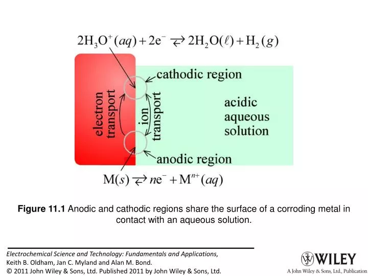
Figure 11.1 Anodic and cathodic regions share the surface of a corroding metal in contact with an aqueous solution.

E N D
Figure 11.1 Anodic and cathodic regions share the surface of a corroding metal in contact with an aqueous solution.
Figure 11.2 A three electrode cell, served by a potentiostat, being used to study a corroding sample of metal. With the switch open, the corrosion potential Ecor is measured. Application of potentials close to Ecor permits a polarization curve to be recorded as in the green curve of Figure 11-3.
Figure 11.3 The upper curve, labelled M is the polarization curve of the metal describing the way in which the net current for metal dissolution depends on the electrode potential. The lower curve, labelled H similarly describes the polarization curve for reaction 11:15. The green curve is the overall current, as directly measurable, equal to the sum of the M and H curves; it crosses zero at the corrosion potential Ecor. The corrosion current Icor reflects the rate of corrosion of the unpolarized metal.
Figure 11.4 Logarithmic presentation of the dependence on electrode potential of the partial currents of the two reactions participating in the corrosion event. The two lines labelled M are the logarithmic magnitudes of the partial currents that sum to the M polarization curve in Figure 11-3. Similarly, the two other lines correspond to the H polarization curve in Figure 11-3. Where the lines are bordered in green, the total current closely approximates the reductive or oxidative partial currents. The slopes of the four lines are –1/brdM, 1/brdM, –1/brdH, and 1/boxH.
Figure 11.7 A graph versus potential of the logarithms of the absolute values of the partial currents for three reactions: 2H3O+ (aq) + 2e–⇄ H2(aq) + H2O(ℓ), Fe(s) ⇄ 2e– + Fe2+(aq), and Zn(s) ⇄ 2e– + Zn2+ (aq). In each case, the oxidative partial current is shown in red and the reductive partial current in blue. The symbols log10{Icor} and Ecor show, for each metal, where the corrosion current and the corrosion potential would have been located in the absence of the other metal. When both metals are present and electrically connected, the corrosion potential is close to that for zinc alone, resulting in a greatly diminished corrosion current for the iron.
Figure 11.8 On progressively making the potential of an iron electrode more positive, corrosion suddenly ceases and the metal becomes passivated.
Figure 11.9 Pourbaix diagram for copper, showing regions in which copper is thermodynamically immune from corrosion, passivated, or liable to corrode.