Download
1 / 38
380 likes | 510 Views
Managing Cloud Resources: Distributed Rate Limiting. Alex C. Snoeren Kevin Webb, Bhanu Chandra Vattikonda , Barath Raghavan , Kashi Vishwanath , Sriram Ramabhadran , and Kenneth Yocum Building and Programming the Cloud Workshop 13 January 2010. Hosting with a single physical presence

E N D
Managing Cloud Resources: Distributed Rate Limiting Alex C. Snoeren Kevin Webb, Bhanu Chandra Vattikonda, BarathRaghavan, KashiVishwanath, SriramRamabhadran,and Kenneth Yocum Building and Programming the Cloud Workshop 13 January 2010
Hosting with a single physical presence However, clients are across the Internet Centralized Internet services Mysore-Park Cloud Workshop – 13 January 2010
Cloud-based services • Resources and clients distributed across the world • Often incorporates resources from multiple providers Windows Live Mysore-Park Cloud Workshop – 13 January 2010
Resources in the Cloud • Distributed resource consumption • Clients consume resources at multiple sites • Metered billing is state-of-the-art • Service “punished” for popularity • Those unable to pay are disconnected • No control of resources used to serve increased demand • Overprovision and pray • Application designers typically cannot describe needs • Individual service bottlenecks varied but severe • IOps, network bandwidth, CPU, RAM, etc. • Need a way to balance resource demand Mysore-Park Cloud Workshop – 13 January 2010
Two lynchpins for success • Need a way to control and manage distributed resources as if they were centralized • All current models from OS scheduling and provisioning literature assume full knowledge and absolute control • (This talk focuses specifically on network bandwidth) • Must be able to efficiently support rapidly evolving application demand • Balance the resource needs to hardware realization automatically without application designer input • (Another talk if you’re interested) Mysore-Park Cloud Workshop – 13 January 2010
Ideal: Emulate a single limiter • Make distributed feel centralized • Packets should experience the same limiter behavior Limiters S D 0 ms S D 0 ms 0 ms S D Mysore-Park Cloud Workshop – 13 January 2010
Accuracy (how close to K Mbps is delivered, flow rate fairness) + Responsiveness (how quickly demand shifts are accommodated) Vs. Communication Efficiency (how much and often rate limiters must communicate) Engineering tradeoffs Mysore-Park Cloud Workshop – 13 January 2010
An initial architecture Limiter 1 Estimate interval timer Limiter 2 Packet arrival Gossip Limiter 3 Enforce limit Estimate local demand Gossip Gossip Limiter 4 Set allocation Global demand Mysore-Park Cloud Workshop – 13 January 2010
Token bucket limiters Packet Token bucket, fill rate K Mbps Mysore-Park Cloud Workshop – 13 January 2010
A global token bucket (GTB)? Demand info (bytes/sec) Limiter 1 Limiter 2 Mysore-Park Cloud Workshop – 13 January 2010
A baseline experiment Limiter 1 3 TCP flows Single token bucket D S 10 TCP flows D S Limiter 2 7 TCP flows S D Mysore-Park Cloud Workshop – 13 January 2010
GTB performance Global token bucket Single token bucket 10 TCP flows 7 TCP flows 3 TCP flows Problem: GTB requires near-instantaneous arrival info Mysore-Park Cloud Workshop – 13 January 2010
Take 2: Global Random Drop Limiters send, collect global rate info from others 5 Mbps (limit) 4 Mbps (global arrival rate) Case 1: Below global limit, forward packet Mysore-Park Cloud Workshop – 13 January 2010
Global Random Drop (GRD) 6 Mbps (global arrival rate) 5 Mbps (limit) Same at all limiters Case 2: Above global limit, drop with probability: Excess / Global arrival rate = 1/6 Mysore-Park Cloud Workshop – 13 January 2010
GRD baseline performance Global token bucket Single token bucket 10 TCPflows 7 TCP flows 3 TCP flows Delivers flow behavior similar to a central limiter Mysore-Park Cloud Workshop – 13 January 2010
GRD under dynamic arrivals Mysore-Park Cloud Workshop – 13 January 2010 (50-ms estimate interval)
Returning to our baseline Limiter 1 3 TCP flows D S Limiter 2 7 TCP flows D S Mysore-Park Cloud Workshop – 13 January 2010
Basic idea: flow counting Goal: Provide inter-flow fairness for TCP flows Local token-bucket enforcement “3 flows” “7 flows” Limiter 1 Limiter 2 Mysore-Park Cloud Workshop – 13 January 2010
Estimating TCP demand Localtoken rate (limit) = 10 Mbps 1 TCP flow S Flow A = 5 Mbps 1 TCP flow S Flow B = 5 Mbps Flow count = 2 flows Mysore-Park Cloud Workshop – 13 January 2010
FPS under dynamic arrivals Mysore-Park Cloud Workshop – 13 January 2010 (500-ms estimate interval)
Comparing FPS to GRD FPS(500-ms est. int.) GRD(50-ms est. int.) • Both are responsive and provide similar utilization • GRD requires accurate estimates of the global rate at all limiters. Mysore-Park Cloud Workshop – 13 January 2010
Estimating skewed demand Limiter 1 1 TCP flow S D 1 TCP flow S Limiter 2 3 TCP flows D S Mysore-Park Cloud Workshop – 13 January 2010
Estimating skewed demand Localtoken rate (limit) = 10 Mbps Flow A = 8 Mbps Bottleneckedelsewhere Flow B = 2 Mbps Flow count ≠ demand Key insight: Use a TCP flow’s rate to infer demand Mysore-Park Cloud Workshop – 13 January 2010
Estimating skewed demand Localtoken rate (limit) = 10 Mbps Flow A = 8 Mbps Bottleneckedelsewhere Flow B = 2 Mbps Local Limit Largest Flow’s Rate 10 8 = 1.25 flows = Mysore-Park Cloud Workshop – 13 January 2010
FPS example Global limit = 10 Mbps Limiter 1 Limiter 2 1.25flows 3flows Global limit x local flow count Total flow count Set local token rate = 10 Mbps x 1.25 1.25 + 3 = = 2.94 Mbps Mysore-Park Cloud Workshop – 13 January 2010
FPS bottleneck example Mysore-Park Cloud Workshop – 13 January 2010 Initially 3:7 split between 10 un-bottlenecked flows At 25s, 7-flow aggregate bottlenecked to 2 Mbps At 45s, un-bottlenecked flow arrives: 3:1 for 8 Mbps
Real world constraints • Resources spent tracking usage is pure overhead • Efficient implementation (<3% CPU, sample & hold) • Modest communication budget (<1% bandwidth) • Control channel is slow and lossy • Need to extend gossip protocols to tolerate loss • An interesting research problem on its own… • The nodes themselves may fail or partition • In an asynchronous system, you cannot tell the difference • Need to have a mechanism that deals gracefully with both Mysore-Park Cloud Workshop – 13 January 2010
Robust control communication Mysore-Park Cloud Workshop – 13 January 2010 7 Limiters enforcing 10 Mbps limit Demand fluctuates every 5 sec between 1-100 flows Varying loss on the control channel
Handling partitions Mysore-Park Cloud Workshop – 13 January 2010 Failsafe operation: each disconnected group k/n Ideally: Bank-o-mat problem (credit/debit scheme) Challege: group membership with asymmetric partitions
Following PlanetLab demand • Apache Web servers on 10 PlanetLab nodes • 5-Mbps aggregate limit • Shift load over time from 10 nodes to 4 5 Mbps Mysore-Park Cloud Workshop – 13 January 2010
Current limiting options Demands at 10 apache servers on Planetlab Wasted capacity Demand shifts to just 4 nodes Mysore-Park Cloud Workshop – 13 January 2010 31
Applying FPS on PlanetLab Mysore-Park Cloud Workshop – 13 January 2010 32
Hierarchical limiting Mysore-Park Cloud Workshop – 13 January 2010
A sample use case Mysore-Park Cloud Workshop – 13 January 2010 • T 0: A: 5 flows at L1 • T 55: A: 5 flows at L2 • T 110: B: 5 flows at L1 • T 165: B: 5 flows at L2
Worldwide flow join Mysore-Park Cloud Workshop – 13 January 2010 • 8 nodes split between UCSD and Polish Telecom • 5 Mbps aggregate limit • A new flow arrives at each limiter every 10 seconds
Worldwide demand shift Mysore-Park Cloud Workshop – 13 January 2010 • Same demand-shift experiment as before • At 50 sec, Polish Telecom demand disappears • Reappears at 90 sec.
Where to go from here • Need to “let go” of full control, make decisions with only a “cloudy” view of actual resource consumption • Distinguish between what you know and what you don’t know • Operate efficiently when you know you know. • Have failsafe options when you know you don’t. • Moreover, we cannot rely upon application/service designers to understand their resource demands • The system needs to dynamically adjust to shifts • We’ve started to manage the demand equation • We’re now focusing on the supply side: custom-tailored resource provisioning. Mysore-Park Cloud Workshop – 13 January 2010