Download
1 / 38
380 likes | 471 Views
Informed Search Problems. CSD 15-780: Graduate Artificial Intelligence Instructors: Zico Kolter and Zack Rubinstein TA: Vittorio Perera. Example of a search tree. How to Improve Search?. Avoid repeated states. Use domain knowledge to intelligently guide search with heuristics.

E N D
Informed Search Problems CSD 15-780: Graduate Artificial Intelligence Instructors: ZicoKolter and Zack Rubinstein TA: Vittorio Perera
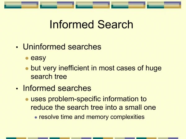
How to Improve Search? • Avoid repeated states. • Use domain knowledge to intelligently guide search with heuristics.
Avoiding repeated states • Do not re-generate the state you just came from. • Do not create paths with cycles. • Do not generate any state that was generated before (using a hash table to store all generated nodes)
What are heuristics? • Heuristic: problem-specific knowledge that reduces expected search effort. • Heuristic functions evaluate the relative desirability of expanding a node. • Heuristics are often estimates of the distance to a goal. • In blind search techniques, such knowledge can be encoded only via state space and operator representation.
Examples of heuristics • Travel planning • Euclidean distance • 8-puzzle • Manhattan distance • Number of misplaced tiles • Traveling salesman problem • Minimum spanning tree Where do heuristics come from?
Heuristics from relaxed models • Heuristics can be generated via simplified models of the problem • Simplification can be modeled as deleting constraints on operators • Key property: Heuristic value can be calculated efficiently
Best-first search 1. Start with OPEN containing a single node with the initial state and a value resulting from applying eval-fn(node). 2. Until a goal is found or there are no nodes on OPEN do: (a) Select the best node on OPEN. (b) Generate its successors. (c) For each successor do:
Best-first search cont. i. If it has not been generated before, evaluate it, add it to OPEN, and record its parent. ii. If it has been generated before, change the parent if this new path is better than the previous one. In that case, update the cost of getting to this node and to any successors that this node may already have (can be avoided when certain conditions hold).
Greedy Best-First Search • Evaluation of each node is h(n). • Selection of next node is nin OPENwith min(h(n)). • Expand until n is the goal, i.e., h(n) = 0.
Time and Space Complexity of Best-first Search • Time Complexity = O(bm) • Space Complexity = O(bm) • High space complexity because nodes are kept in memory to update paths. • These are worst-case complexities. A good heuristic substantially reduces them.
Problems with best-first search • Uses a lot of space • The resulting algorithm is complete but not optimal • Complete if no infinite path explored. • Analogy: water • Problem: rivers are not the shortest path
Minimizing total path cost: A* • Similar to best-first search except that the evaluation is based on total path (solution) cost: f(n) = g(n) +h(n) where: g(n) =cost of path from the initial state to n h(n) =estimate of the remaining distance
Admissibility and Monotonicity • Admissible heuristic = never overestimates the actual cost to reach a goal. • Monotone heuristic = the f value never decreases along any path. • When h is admissible, monotonicity can be maintained when combined with pathmax: f(n) = max(f(n), g(n)+h(n))
Optimality of A* Intuitive explanation for monotone h: • If h is a lower-bound, then f is a lower-bound on shortest-path through that node. • Therefore, f never decreases. • It is obvious that the first solution found is optimal (as long as a solution is accepted when f(solution) f(node) for every other node).
Proof of optimality of A* Let O be an optimal solution with path cost f*. Let SO be a suboptimal goal state, that is g(SO) >f* Suppose that A* terminates the search with SO. Let n be a leaf node on the optimal path to O f* ≥ f(n)admissibility ofh f(n) ≥ f(SO)n was not chosen for expansion f* ≥ f(n) ≥ f(SO) f(SO) = g(SO)SO is a goal, h(SO) = 0 f* ≥ g(SO)contradiction!
Completeness of A* A* is complete unless there are infinitely many nodes with f(n) < f* A* is complete when: (1) there is a positive lower bound on the cost of operators. (2) the branching factor is finite.
A* is maximally efficient • For a given heuristic function, no optimal algorithm is guaranteed to do less work. • Aside from ties in f, A* expands every node necessary for the proof that we’ve found the shortest path, and no other nodes.
Measuring the heuristics payoff • The effective branching factor b* is: N = 1 + b* + (b*)2 + ... + (b*)d • Domination among heuristic functions
Measuring the Heuristics Payoff (cont.) • h2 dominates h1 is if, for any node n, h2(n)h1(n) • As long as h2 does not overestimate. • Intuition: The higher value represents a closer approximation to the actual cost of the solution. Therefore, less states are expanded.
Time and Space Complexity of A* Search • Time Complexity = exponential unless the error in the heuristic function is less than or equal to the logarithm of the actual path cost. • |h(n) – h*(n)| O(log h*(n)) • Space Complexity = O(bm) • High space complexity because all generated nodes are kept in memory. • These are worst-case complexities. A good heuristic substantially reduces them.
Search with limited memory Problem: How to handle the exponential growth of memory used by admissible search algorithms such as A*. Solutions: • IDA* [Korf, 1985] • SMA* [Russell, 1992] • RBFS [Korf, 1993]
IDA* - Iterative Deepening A* • Beginning with an f-bound equal to the f-value of the initial state, perform a depth-first search bounded by the f-bound instead of a depth bound. • Unless the goal is found, increase the f-bound to the lowest f-value found in the previous search that exceeds the previous f-bound, and restart the depth first search.
Advantages of IDA* • Use depth-first search with f-cost limit instead of depth limit. • IDA* is complete and optimal but it uses less memory [O(bf*/)] and more time than A*.
SMA* • Utilizes whatever memory is available. • Avoids repeated states as far as memory allows. • Complete if the available memory is sufficient to store the shallowest solution path. • Returns the best solution that can be reached with the available memory. • Optimal if enough memory is available to store the shallowest optimal solution path. • Optimally efficient when enough memory is available for the entire search tree.
SMA* cont. A 0+12=12 10 8 B G 10+5=15 8+5=13 8 16 10 10 C D H I 20+5=25 20+0=20 16+2=18 24+0=24 10 10 8 8 E F J K 30+5=35 30+0=30 24+0=24 24+5=29
SMA* cont. A A A A 13(15) 12 12 13 B B G G 13 13 15 15 H 18 inf
SMA* cont. A A A A 15(15) 15(24) 20(24) 15 G B B G B 24(inf) 20(inf) 15 15 24 I C D 25 inf 20 24