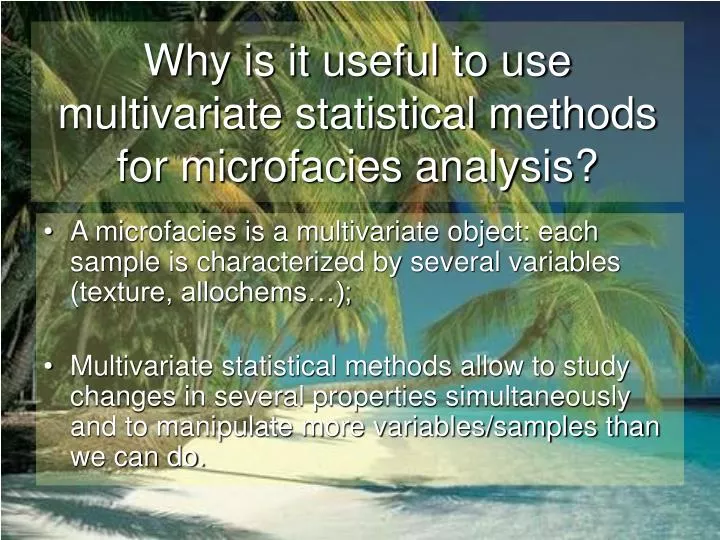
Why is it useful to use multivariate statistical methods for microfacies analysis?

1. Why is it useful to use multivariate statistical methods for microfacies analysis? • A microfacies is a multivariate object: each sample is characterized by several variables (texture, allochems…); • Multivariate statistical methods allow to study changes in several properties simultaneously and to manipulate more variables/samples than we can do.

2. CLUSTER ANALYSIS(hierarchical, agglomerative)

3. Basics • Grouping of objects (samples) based on similarity or difference of their variables (components) > Q-mode (R-mode = variables); • Reduces the dimensionality of your (multivariate) data table; • Matrix of similarity coefficients: numerical similarity between all pairs of objects.

4. Procedure • Select variables (mixing different types is not adviced!); • Calculate distance/similarity between all samples (= initial ‘clusters’) and store in a distance matrix (= similarity matrix); • Select the two most similar initial clusters (samples) in the matrix and fuse them; • Calculate the distance between that new cluster and all others (mono-sample). Only the distances involving that cluster will have changed, no need to re-calculate all distances; • Repeat 3 until all samples are in one cluster.

5. Similarity measures • Distance coefficients: 2 main types, Euclidian or not (e.g. Manhattan); • Correlation similarity coefficient; • Association coefficients (only for binary 1-0 data).

6. 1. Distance coefficients • Data = scatter of points (samples) in a multidimensional space (components of a microfacies) > distance = (dis-)similarity. n = component

7. A d A-B = (xB-xA)2 + (yA-yB)2 B m d A-B = S(iB-iA)2 i=1 Euclidian = straight line (hypo.) 2D y x mD 3D Or to avoid the measure to increase with more variables: m d A-B = 1/m S(iB-iA)2 i=1

8. Manhattan = sum 2D A d A-B = 1/2 I xB-xA I + I yA-yB I y B x mD m d A-B = 1/m SI iB-iA I i=1 According to some, more robust to outliers.

9. Remarks: • Euclidian distance is intuitive but underestimates joint differences, ex. 2 shape characters of an organism should be regarded as due to 2 separate genetic changes, so the real difference between them is the sum of the differences, not the length of the hypothenuse. So the choice between Euclidian or Manhattan is fct of the independence of variables in the causative process: do 2 differences really mean 2x the difference or just 2 linked consequences of 1 difference?

10. Remarks: • Standardisation prior to distance calculation: units / scale. Euclidian distance = (6002 + 0.82) = 600,005 ex. force both in 0-1 = 0.6 and 0.8 Even when units are the same, a small variation in one variable might be geologically as important as a large variation in another!

11. And… • Distance measures are dependent on the magnitude of the variables, not always desirable… • Ex.a: 2 fossils may be identical in shape [correlation] but have very different sizes [distances] > in this case we might want to regard similarity in terms of ratios between variable values. • Ex.b: Two biostratigraphic samples are more similar if the relative proportions of species are similar [correlation] or if abundances (counts) of the species are similar [distances]?

12. 2. Correlation similarity coefficients • Uses Pearson’s correlation coefficient r but instead of many objects (samples) and 2 variables (components) we have two objects and many variables > scatter plot with axes = samples and data points are variables. • Standardisation is less important in this case but outliers can affect strongly the results (high or low values in one or two variable).

13. 3. Association coefficients • For binary data (microfacies, palaeontology); • A and B are compared on the basis of a contingency matrix: sample B a to d are number of variables present absent present a b sample A absent c d

14. There is a large variety of association coefficients calculated on a, b, c and d designed to do well according to various criteria. Here are two common examples: a Jaccard: JAB = a + b + c Joint absences (d) are not considered as indicative of similarity 2a Dice-Sorensen: DAB = 2a + b + c More weight is given to joint-presences

15. In PAST 1.33 • Various measures are proposed to build the matrix of similarity: • Euclidian (robust) and Manhattan; • Correlation using r; • Dice-Sorensen, Jaccard, Simpson, Raup-Crick for presence/absence; • Various for abundances (Bray-Curtis, Cosine, Chord, Morisita, Horn); • Hamming for categorical data.

16. Clustering algorithms • Divise methods = find the sparse areas for positioning boundaries between clusters; • Density methods = multivariate space is searched for concentrations of points; • Linkage methods = nearby points are iteratively linked together.

17. Common methods (linkage) A. Nearest-neighbour = single linkage: similarity between one point and a new cluster (or 2 clusters) = similarity between that point and the most similar point in the cluster less than true distance for most points so easy for points to link on to the ends of dispersed, elongated clusters with points at oppsite ends substantially different (has been widely used in numerical taxonomy)

18. Nearest neighbour

19. Common methods (linkage) B. Furthest-neighbour = complete linkage: similarity between one point and a new cluster (or 2 clusters) = weakest of all candidate pairwise similarities, greatest distance apparent interclusters distances maximised, tends to produce very tight clusters of similar cases, sometimes breaking up ‘too far’

20. Furthest neighbour

21. Common methods (linkage) similarity between one point and a new cluster (or 2 clusters) = average (many different ways) C. Average linkage: Most common: Unweighted Pair-Groups Method Average (UPGMA) = average distance is calculated from the distance between each point in a cluster and all other points in another cluster. The two clusters with the lowest average distance are joined together to form the new cluster.

22. Common methods (linkage) D. Ward’s method: Linkage such that there is the least increase in the sum of squared deviations from the cluster means in order to control the increase in variance of clusters during linkage. The criterion for fusion is that it should produce the smallest possible increase in the error sum of squares. Good looking and well-proportioned so became de facto standard… Works only with euclidian distance.

23. Ward’s method phenon line

24. Dendrogram • Result of the analysis = ordered series of linkages between clusters, each at a specific magnitude of similarity. Best represented graphically by a dendrogram; • The phenon line cuts the structure at a chosen level to isolate meaningful clusters. Indeed all clusters will be linked ultimately by the method; • Where to draw that line is based on: pragmatic requirements, preconceptions (if the number of categories is not itself under investigation) and ‘natural’ divisions if they exist (gaps, jumps).

25. ‘natural division’

26. Example samples euclidian distance in 2 variables space

28. How good is cluster analysis? • Objective classification but with (most often) subjective choices at many levels; Same data > very different (valid) results; • New observations will modify the clusters, sometimes strongly > instabilty; • No available test for difference from random population; • « profound conclusions should not be based on such uncertain foundations » Swan & Sandilands (1995). • Test various clustering methods on your data and see if results are comparable!! Remove isolated outliers prior to analysis. • Average linkage seems to offer the best stability for clusters.

29. References • PAST: http://folk.uio.no/ohammer/past/ • Good websites: - http://149.170.199.144/multivar/ca.htm - http://www.statsoft.com/textbook/stcluan.html - http://www2.chass.ncsu.edu/garson/pa765/cluster.htm Very good reference for data analysis in geology: Swan, A.R.H. & Sandilands, M. 1995. Introduction to geological data analysis. Blackwell Science.