Download

1 / 49
500 likes | 689 Views
Removing Ill-posedness in Numerical Computation ---- GCD, JCF and Multiple Roots. Zhonggang Zeng. April 20, 2004, University of Notre Dame. Ill-posed problems are common in applications. image restoration - deconvolution IVP for stiction damped oscillator - inverse heat conduction

E N D
Removing Ill-posedness in Numerical Computation ---- GCD, JCF and Multiple Roots Zhonggang Zeng April 20, 2004, University of Notre Dame
Ill-posed problems are common in applications • image restoration - deconvolution • IVP for stiction damped oscillator - inverse heat conduction • some optimal control problems - electromagnetic inverse scatering • air-sea heat fluxes estimation - the Cauchy prob. for Laplace eq. • … … • A well-posed problem: (Hadamard) • the solution satisfies • existence • uniqueness • continuity w.r.t data 1
Ill-posed problems in numerical analysis • matrix rank-revealing - overdetermined system • - multivariate polynomial factoring - polynomial GCD • Jordan Canonical Form - multiple zeros and eigenvalues • - nonisolated zeros … … Can you solve (x-1.0)100 = 0 x100-100 x99 +4950 x98 - 161700 x97+3921225x96 - ... - 100 x +1 = 0 -2-
Exact roots 1.072753787571903102973345215911852872073… 0.422344648788787166815198898160900915499… 0.422344648788787166815198898160900915499… 2.603418941910394555618569229522806448999… 2.603418941910394555618569229522806448999 … 2.603418941910394555618569229522806448999 … 1.710524183747873288503605282346269140403… 1.710524183747873288503605282346269140403… 1.710524183747873288503605282346269140403… 1.710524183747873288503605282346269140403… Inexact coefficients 2372413541474339676910695241133745439996376 -21727618192764014977087878553429208549790220 83017972998760481224804578100165918125988254 -175233447692680232287736669617034667590560780 228740383018936986749432151287201460989730170 -194824889329268365617381244488160676107856140 110500081573983216042103084234600451650439720 -41455438401474709440879035174998852213892159 9890516368573661313659709437834514939863439 -1359954781944210276988875203332838814941903 82074319378143992298461706302713313023249 “attainable” roots 1.072753787571903102973345215911852872073… 0.422344648788787166815198898160900915499… 0.422344648788787166815198898160900915499… 2.603418941910394555618569229522806448999… 2.603418941910394555618569229522806448999 … 2.603418941910394555618569229522806448999 … 1.710524183747873288503605282346269140403… 1.710524183747873288503605282346269140403… 1.710524183747873288503605282346269140403… 1.710524183747873288503605282346269140403… 9 3 5 5 Exact coefficients 2372413541474339676910695241133745439996376 -21727618192764014977087878553429208549790220 83017972998760481224804578100165918125988254 -175233447692680232287736669617034667590560789 228740383018936986749432151287201460989730173 -194824889329268365617381244488160676107856145 110500081573983216042103084234600451650439725 -41455438401474709440879035174998852213892159 9890516368573661313659709437834514939863439 -1359954781944210276988875203332838814941903 82074319378143992298461706302713313023249 -3-
“attainable” roots 1.072753787571903102973345215911852872073… 0.422344648788787166815198898160900915499… 0.422344648788787166815198898160900915499… 2.603418941910394555618569229522806448999… 2.603418941910394555618569229522806448999 … 2.603418941910394555618569229522806448999… 1.710524183747873288503605282346269140403… 1.710524183747873288503605282346269140403… 1.710524183747873288503605282346269140403… 1.710524183747873288503605282346269140403… Coeff. in hardware precision 2372413541474339676910695241133745439996376 -21727618192764014977087878553429208549790220 83017972998760481224804578100165918125988254 -175233447692680232287736669617034667590560789 228740383018936986749432151287201460989730173 -194824889329268365617381244488160676107856145 110500081573983216042103084234600451650439725 -41455438401474709440879035174998852213892159 9890516368573661313659709437834514939863439 -1359954781944210276988875203332838814941903 82074319378143992298461706302713313023249 The multiplicity structure[1,2,3,4] becomes[1,1,1,1,1,1,1,1,1,1] ----- typical ill-posedness The highest multiplicity is only 4! -4-
The computed roots: + + + + For polynomial with coefficients in hardware precision: -5-
GCD( f, g )= Under tiny perturbation: -6-
Every eigenvalue corresponds to a Jordan structure l 1 l 1 l AX = X l 1 l l 1 l l3 l4 l2 l Under arbitrary perturbation l5 l l1 l8 l1 l6 l2 l7 l3 l4 -- nearly rank deficient l5 l6 l7 l8 Jordan Canonical Form (JCF) l3 -7-
The challenge: Ill-posed problem in numerical computation - data error is common in application - round-off error is inevitable - Ill-posedness ill-condition to the extreme -8-
James H. Wilkinson (1919-1986) Backward error and condition number won 1970 Turing Award for backward error analysis Numerical Computation seeks The exact solution of a nearby problem -9-
Ill-posedness is incompatible with numerical compuation Backward and forward error -10-
From problem From computational method The condition number [Forward error] < [Condition number] [Backward error] A large condition number <=> The problem is sensitiveor, ill-conditioned An ill-posed problem ==> condition number is infinity -11-
If the answer is highly sensitive to perturbations, you have probably asked the wrong question. Maxims about numerical mathematics, computers, science and life, L. N. Trefethen. SIAM News A: “Customer” B: Numerical analyst Who is asking a wrong question? A: The polynomial, matrix B: The computing objective What is the wrong question? -12-
The question we used to ask: (in root-finding) (Fundamental Theorem of Algebra) Given a polynomial p(x) = xn + a1 xn-1+...+an-1 x + an find z = (z1, ..., zn)such that p(x) = ( x - z1)( x - z2) ... ( x - zn ) This problem is ill-posed when multiple roots exist -13-
William Kahan: This is a misconception Are multiple roots really sensitive to perturbations? Kahan’s discovery in 1972: multiple roots are sensitive to arbitrary perturbation, but insensitive to multiplicity preserving perturbation. -14-
Kahan’s pejorative manifolds All n-polynomials having certain multiplicity structure form a pejorative manifold xn + a1xn-1+...+an-1 x + an<=> (a1, ..., an-1 , an) Example: ( x-t)2 = x2 + (-2t) x + t2 Pejorative manifold: a1= -2t a2= t2 -15-
Pejorative manifolds of 3rd-degree polynomials ( x - s)( x - t)2 = x3 + (-s-2t) x2 + (2st+t2) x + (-st2) a1= -s-2t a2= 2st+t2 a3= -st2 Pejorative manifold of multiplicity structure [1,2] ( x - s)3 =x3 + (-3s) x2 + (3s2) x + (-s3) a1 = -3s a2 = 3s2 a3 = -s3 Pejorative manifold of multiplicity structure [ 3 ] -16-
Pejorative manifolds of degree 3 polynomials The wings: a1= -s-2t a2= 2st+t2 a3= -st2 The edge: a1 = -3s a2 = 3s2 a3 = -s3 General form of pejorative manifolds u = G(z) -17-
W. Kahan, Conserving confluence curbs ill-condition, 1972 • Ill-condition occurs when a polynomial is near a pejorative manifold. • Roots are not necessarily sensitive when the polynomial stay • on that pejorative manifold Ill-condition is caused by solving a polynomial equation on a wrong manifold Although Kahan did not propose a practical algorithm, this unpublished work provides a valuable insight on ill-condition and ill-posedness -18-
For the ill-posed multiple root problem with inexact data The key: Remove the ill-posedness by reformulating the problem Original problem: calculating the roots Reformulated problem: finding the nearest polynomial on a proper pejorative manifold -- A constraint minimization Z. Zeng, Computing multiple roots of inexact polynomials, to appear, Math Comp -19-
perturbed polynomial p P original polynomial pejorative manifold Minimize q projected polynomial with computed roots Illustration of the reformulated problem: • q has the same multiplicity structure as p • roots of q are accurate approximation to those of p -20-
(m<n) (degree) n m (number of distinct roots) To calculate roots of p(x)= xn + a1xn-1+...+an-1 x + an Let ( x - z1 ) l1( x - z2) l2 ... ( x - zm) lm = xn + g1( z1, ..., zm )xn-1+...+gn-1( z1, ..., zm ) x + gn( z1, ..., zm ) Then, p(x) = ( x - z1 ) l1( x - z2) l2 ... ( x - zm) lm <==> g1( z1, ..., zm )=a1 g2( z1, ..., zm )=a2 ... ... ... gn( z1, ..., zm )=an I.e. An over determined polynomial system G(z) = a -21-
The coefficient operator: Its Jacobian: , Theorem: J(z) is of full rank <=> z1,…,zm are distinct. Or the decomposition ( x - z1 ) l1( x - z2) l2 ... ( x - zm) lm is unreducible -22-
v = G(z) u = G(y) forward error (on roots) backward error (on data) condition number Definition: The structure-preserving condition number: The structure-preserving condition number
given polynomial b ~ q(x) a original polynomial Gl(z) = a ~ p b computed polynomial It is now a well-posed problem! -24-
At multiple roots, condition number = Example: Conventional sensitivity measurement: Structure preserving sensitivity measurement: Multiple roots may not be sensitive after all! After removing ill-posedness, we also removed ill-condition -25-
pejorative manifold a Minimize ||G(z)=a ||2 u=G(z) Question: How to solve the reformulated problem: An overdetermined system for its least squares solution -26-
Project to tangent plane u1 = G(z0)+J(z0)(z1- z0) ~ tangent plane P0 : u = G(z0)+J(z0)(z- z0) pejorative root u*=G(z*) new iterate u1=G(z1) initial iterate u0=G(z0) The polynomial a Pejorative manifold u = G( z ) Solve G( z ) = a for nonlinear least squares solutionz=z* Solve G(z0)+J(z0)(z - z0 ) = a for linear least squares solutionz =z1 G(z0)+J(z0)(z - z0 ) = a J(z0)(z - z0 ) = - [G(z0) - a ] z1 = z0 - [J(z0)+][G(z0) - a] -27-
The Gauss-Newton iteration z (i+1)=z(i) - J(z(i))+[ G(z (i)) - a ], i=0,1,2 ... where J(.)+ is the pseudo-inverse of J(.) • Theorem: The Gauss-Newton iteration locally converges • at quadratic rate if the polynomial is exact • at linear rate if the polynomial is inexact but close -28-
multiplicity structure initial iterate on Algorithm: Given Apply the Gauss-Newton iteration z (i+1)=z(i) - J(z(i))+[ Gl(z (i)) - a ], i=0,1,2 ... As a well-posed and well conditioned problem, multiple roots can be calculated accurately -29-
distinct roots: u0(x) = [(x-1)4(x-2) 2] [(x-1)(x-2)(x-3)] * * * u1(x) = [(x-1)3(x-2) ] [(x-1)(x-2)] * * u2(x) = [(x-1)2] [(x-1)(x-2)] * * u3(x) = [(x-1)] [(x-1)] * u4(x) = [1] [(x-1)] * ----------------------------------------- multiplicities 5 3 1 Identifying the multiplicity structure p(x)= (x-1)5(x-2) 3(x-3) = [(x-1)4(x-2) 2] [(x-1)(x-2)(x-3)] p’(x)= [(x-1)4(x-2) 2][ (x-1)(x-2)+5(x -2)(x -3)+3(x -1)(x -3)] GCD(p,p’) = [(x-1)4(x-2) 2] u0 = p um =GCD(um-1, um-1’) -30-
the key with vj’s being squarefree Output : f = v1 v2 … vk - The multiplicity structure A squarefree factorization of f: u0 =f for j = 0, 1, … while deg(uj) > 0 do uj+1 = GCD(uj, uj’) vj+1 = uj/uj+1 end do - The number of distinct roots: m = deg(v1) - Roots of vj’s are initial approximation to the roots of f -31-
For given polynomials f and g, find u, v, w such that which is an important application problem in its own right. Applications: Robotics, computer vision, image restoration, control theory, system identification, canonical transformation, mechanical geometry theorem proving, hybrid rational function approximation … … Root-finding leads to another ill-posed problem: The Approximate GCD of inexact polynomials. Part I: a univariate algorithm, Z. Zeng The Approximate GCD of inexact polynomials. Part II: a multivariate algorithm, Z. Zeng and B. Dayton -32-
Where : coefficient vectors : convolution matrices Again, the key: Remove ill-posedness by reformulating the problem If the degree of u = GCD(f,g) is known: -33-
Define GCD-finding overdetermined system Minimize Reformulated problem: (a least squares problem) -34-
For the problem with The Jacobian Minimize Theorem: The Jacobian is of full rank if v and w are co-prime --- ill posedness is removed! -35-
perturbed polynomial pair pejorative manifold perturbed polynomial pair original polynomial pair (f,g) projected polynomials with computed GCD Illustration of the reformulated problem: Again, the problem becomes well-posed, and often well-conditioned! -36-
Or, solve in least squares sense is full-ranked • The Gauss-Newton iteration locally converges Given a polynomial pair ( f, g ) Problem: Find u = GCD( f, g ). --- ill-posed Reformulated problem: Find a pair (p, q) = (uv, uw)that is nearest to ( f, g ) s.t. a constrainton the degree of u = GCD( p, q ) • Condition number is finite -37-
If then The Sylvester Resultant matrix is approximately rank-deficient The GCD structure is determined by computing the approximate rank of Sylvester matrices A rank-revealing method and its applications, T. Y. Li and Z. Zeng, to appear: SIMAX The question: How to determine the GCD structure
S2(f,g) S1(f,g) = QR QR until finding the first rank-deficient Sylvester submatrix by formulating and the Gauss-Newton iteration For univariate polynomials : Stage I: determine the GCD degree Stage II: determine the GCD factors ( u, v, w ) -39-
by formulating and the Gauss-Newton iteration For multivariate polynomials ( f, g ): Stage I: determine the GCD degrees by applying the univariate GCD on each variable, with other variable randomly fixed. Stage II: determine the GCD factors ( u, v, w ) -40-
Stage I: determine the multiplicity structure Stage II: determine multiple roots by formulating and the Gauss-Newton iteration Back to multiple root computation: by squarefree factorization of f via recursive GCD-finding -41-
Stage II results: The backward error: 6.16 x 10⁻¹⁶ Computed roots multiplicities 1.000000000000000 20 2.999999999999997 15 3.000000000000011 10 3.999999999999985 5 For polynomial with (inexact ) coefficients in machine precision Stage I results: The backward error: 6.05 x 10⁻¹⁰ Computed roots multiplicities 1.000000000000353 20 2.000000000030904 15 3.000000000176196 10 4.000000000109542 5 -42-
For a problem (data ----> solution) with data D0 minimize A two-stage strategy for removing ill-posedness: Stage I: determine the structureSof the desired solution this structure determines a pejorative manifold of data P = P-1(S) = {D | P(D) = S fits the structure } Stage II: formulate and solve a least squares problem by the Gauss-Newton iteration -43-
The two-stage approach leads to Blackbox-type algorithms and software • rank-revealing algorithm • A rank-revealing method and its applications, T. Y. Li and Z. Zeng • univariate GCD algorithm • The approximate GCD of inexact polynomials. Part I: a univariate algorithm, • Z. Zeng • multivariate GCD algorithm • The approximate GCD of inexact polynomials. Part II: a multivariate algorithm, • Z. Zeng and B. H. Dayton • multiple root algorithm • Computing multiple roots of inexact polynomials, Z. Zeng • (Distinguished Paper Award, ISSAC 2003) -44-
l 1 l 1 l JCF structure: [3,2,2,1] l 1 l J = l 1 l l staircase structure: [4,3,1] l l l l + + + + + + + + + + + + + + + + S= l l l + + + l Computing the approximate JCF (joint work with T. Y. Li) Given A, find X, J: AX = XJ Given A, find U, S AU = US -45-
Or, solve an overdetermined system in least squares sense Find U and S that minimize||AU-US ||F subject to UTU = I, E U = O S has a staircase structure Reformulated problem: (constraint minimization) Theorem: If A is near a matrix that has an eigenvalue exactly corresponds to staircase block S, then the Jacobian of H(U,S) is of full rank. --- ill-posedness is removed! --- theGauss-Newton iteration locally converges! -46-
A two-stage strategy for computing JCF: Stage I: determine the Jordan structure and initial approximation to the eigenvalues Stage II: Solve the reformulated minimization problem at each eigenvalue, subject to the structural constraint, using the Gauss-Newtion iteration. -47-
Conclusion: - Ill-posed problems may be reformulated as well-posed and well conditioned ones - A two stage approach may help solving the problem accurately: -- determine the structure -- solve a constraint minimization -48-