Download
1 / 50
500 likes | 514 Views
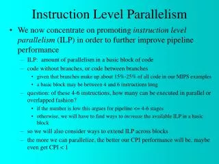
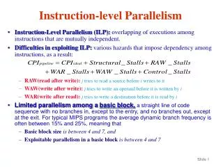
Instruction-level Parallelism. Instruction-Level Parallelism (ILP): overlapping of executions among instructions that are mutually independent. Difficulties in exploiting ILP: various hazards that impose dependency among instructions, as a result:

E N D
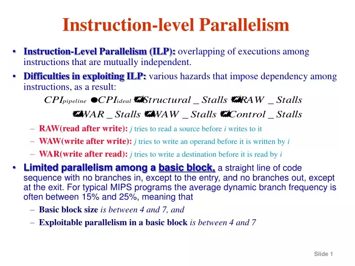
Instruction-level Parallelism • Instruction-Level Parallelism (ILP):overlapping of executions among instructions that are mutually independent. • Difficulties in exploiting ILP:various hazards that impose dependency among instructions, as a result: • RAW(read after write):j tries to read a source before i writes to it • WAW(write after write): j tries to write an operand before it is written by i • WAR(write after read): j tries to write a destination before it is read by i • Limited parallelism among a basic block,a straight line of code sequence with no branches in, except to the entry, and no branches out, except at the exit. For typical MIPS programs the average dynamic branch frequency is often between 15% and 25%, meaning that • Basic block size isbetween 4 and 7, and • Exploitable parallelism in a basic block is between 4 and 7
Instruction-level Parallelism • Loop-Level Parallelism: for (i=1; i<=1000; i=i+1) x[i]=x[i]+ y[i]; • Loop unrolling: static or dynamic, to increase ILP; • Vector instructions: a vector instruction operates on a sequence of data items (pipelining data streams): Load V1, X; Load V2, Y; Add V3,V1,V2; Store V3, X • Data Dependences:an instruction j is data dependent on instruction i if either • instruction i produces a result that may be used by instruction j, or • instruction j isdata dependent on instruction k, and instruction k is data dependent on instruction i. • Dependences are a property of programs, whether a given dependence results inan actual hazard being detected and whether that hazard actually causes a stall are properties of the pipeline organization. • Data Hazards: data dependence vs. name dependence • RAW(real data dependence): j tries to read a source before i writes to it • WAW(output dependence): j tries to write an operand before it is written by i • WAR(antidependence): j tries to write a destination before it is read by i
Instruction-level Parallelism • Control Dependence:determines the ordering of instruction i with respect to a branch instruction so that the instruction is executed in the correct program order and only when it should be. There are two constraints imposed by control dependences: • An instructionthat is control dependent on a branch cannot be moved before the branch so that its execution is no longer controlled by the branch: if p1{ s1; s1; cannot be changed to if p1{ }; }; • An instructionthat is not control dependent on a branch cannot be moved after the branch so that its execution is controlled by the branch: s1; if p1{ if p1{ cannot be changed to s1; }; };
Instruction-level Parallelism • Control Dependences:preservation of control dependence can be achieved by ensuring that instructions execute in program order and the detection of control hazards guarantees an instruction that is control dependent on a branch delays execution until the branch’s direction is known. • Control dependence in itself is not the fundamental performance limit; • Control dependence is not the critical property that must be preserved; instead, the two properties critical to program correctness and normally preserved by maintaining both data and control dependence are: • The exception behavior – any change in the ordering of instruction execution must not change how exceptions are raised in the program (or cause any new exceptions) • The data flow – the actual flow of data values among instructions that produce results and those that consume them.
Examples: DADDU R2,R3,R4 no d-dp prevents BEQZ R2,L1 this exchange LW R1,0(R2) Mem. exception L1: may result ----------------------------------------------- DADDU R1,R2,R3 BEQZ R4,L DSUBU R1,R5,R6 L: ……. OR R7,R1,R8 Preserving data dependence alone is not sufficient for program correctness ‘cause multiple predecessors Speculation, which helps with the exception problem, can lessen impact of control dependence (to be elaborated later) DADDU R2,R3,R4 LW R1,0(R2) BEQZ R2,L1 L1: ------------------------------------------- DADDU R1,R2,R3 BEQZ R12,SN speculation DSUBU R4,R5,R6 DADDU R5,R4,R9 SN: OR R7,R8,R9 The move is okay if R4 is dead after SN, i.e. if R4 is unused after SN, and DSUBU can not generate an exception, because dataflow cannot be affected by this move. Instruction-Level Parallelism
Instruction-Level Parallelism • Dynamic Scheduling: • Advantages • Handles some cases where dependences are unknown at compile time • Simplifies compiler • Allows code that was compiled with one pipeline in mind to run efficiently on a different pipeline • Facilitates hardware speculation • Basic idea: • Out-of-order execution tries to avoid stalling in the presence of detected dependences (that could generate hazards), by scheduling otherwise independent instructions to idle functional units on the pipeline; • Out-of-order completion can result from out-of-order execution; • The former introduces the possibility of WAR and WAW (non-existing in the 5-depth pipeline), while the latter creates major complications in handling exceptions.
Out-of-order execution introduces WAR, also called antidependence, and WAW, also called output dependdnece: DIV.D F0,F2,F4 ADD.D F6,F0,F8 SUB.D F8,F10,F14 MUL.D F6,F10,F8 These hazards are not caused by real data dependences, but by virtue of sharing names! Both of these hazards can be avoided by the use of register renaming Out-of-order completion in dynamic scheduling must preserve exception behavior Exactly those exceptions that would arise if the program were executed in strict program order actually do arise, also called precise exception; Dynamic scheduling may generate imprecise exceptions The processor state when an exception is raised does not look exactly as if the instructions were executed in the strict program order Two reasons for impreciseness: The pipeline may have already completed instructions that are later in program order than the faulty one; and The pipeline may have not yet completedsome instructions that are earlier in program order than the faulty one. Instruction-Level Parallelism
Instruction-Level Parallelism • Out-of-order execution is made possible by splitting the ID stage into two stages, as seen in scoreboard: • Issue – Decode instructions, check for structural hazards. • Read operands – Wait until no data hazards, then read operands. • Dynamic scheduling using Tomasulo’s Algorithm: • Tracks when operands for instructions become available and allow pending instructions to execute immediately, thus minimizing RAW hazards; • Introduces register renaming to minimize the WAW and WAR hazards. DIV.D F0,F2,F4 DIV.D F0,F2,F4 ADD.D F6,F0,F8 use temp reg. S & T ADD.D S,F0,F8 S.D F6,0(R1) to rename F6 & F8 S.D S,0(R1) SUB.D F8,F10,F14 SUB.D T,F10,F14 MUL.D F6,F10,F8 MUL.D F6,F10,T
Instruction-Level Parallelism • Dynamic scheduling using Tomasulo’s Algorithm: • Register renaming in Tomasulo’s scheme is implemented by reservation stations From instruction unit FP registers Instruction queue L/S Ops FP operations Address unit Operand buses Load buffers Store buffers Operation bus 1 Reservation stations 1 2 2 3 Data Address Common data bus (CDB) Memory unit FP adders FP multipliers
Instruction-Level Parallelism • Distinguishing Features of Tomasulo’s Algorithm: • It is a technique allowing execution to proceed in the presence of hazards by means of register renaming. • It uses reservation stations to buffer/fetch operands whenever they become available, eliminating the need to use registers explicitly for holding (intermediate) results. When successive writes to a register take place, only the last one will actually update the register. • Register specifiers (of pending operands) for an instruction are renamed to names of the (corresponding) reservation stations in which the producer instructions reside. • Since there can be more “conceptual” (or logical) reservation stations than there are registers, a much larger “virtual register set” is effectively created. • The Tomasulo method contrasts to the scoreboard method in that the former is decentralized while the latter is centralized. • In the Tomasulo method, a newly generated result is immediately made known and available to all reservation stations (thus all issued instructions) simultaneously, hence avoiding any bottleneck.
Instruction-Level Parallelism • Three Main Steps of Tomasulo’s Algorithm: • Issue: If there is no structural hazards for the current instruction Thenissue the instruction Elsestalluntil structural hazards are cleared. (no WAW hazard checking) • Execute: If both operands are available (no RAW hazards) Thenexecutethe operation Elsemonitorthe Common Data Bus (CDB) until the relevant value (operand) appears on CDB, and then readthe value into the reservation station. When both operands become available in the reservation station, execute the operation. (RAW is cleared as soon as the value appears on CDB!) • Write Result: When result is generated placeit on CDB through which register file and any functional unit waiting on it will be able to read immediately.
Instruction-Level Parallelism • Main Content of A Reservation Station:
Instruction-Level Parallelism • Updating Reservation Stations during the 3 Steps:
Instruction-Level Parallelism • Updating Reservation Stations during the 3 Steps (cont’d):
Instruction-Level Parallelism • An Example of Tomasulo’s Algorithm:when all issued but only one completed
Instruction-Level Parallelism • An Example of Tomasulo’s Algorithm:when MUL.D is ready to write its result
Instruction-Level Parallelism • Another Example of Tomasulo’s Algorithm:multiplying an array by a scalar F2 Note: integer ALU ops (DADDUI R1,R1,-8 & BNE R1,R2,Loop) are ignored and branch is predicted taken.
Instruction-Level Parallelism • The Main Differences between Scoreboard & Tomasulo’s: • In Tomasulo, there is no need to check WAR and WAW (as must be done in Scoreboard) due to renaming, in the form of reservation station number (tag) and load/store buffer number (tag). • In Tomasulo pending result (source operand in case of RAW) is obtained on CDB rather than from register file. • In Tomasulo loads and stores are treated as basic functional unit operations. • In Tomasulo control is decentralizedrather than centralized -- data structures for hazard detection and resolution are attached to reservation stations, register file, or load/store buffers, allowing control decisions to be made locally at reservation stations, register file, or load/store buffers.
Instruction-Level Parallelism • Summary of the Tomasulo Method: • The order of load and store instructions is no longer important so long as they do not refer to the same memory address. Otherwise conflicts on memory locations are checked and resolved by the store buffer for all items to be written. • There is a relatively high hardware cost: • associative search for matching in the reservation stations • possible duplications of CDB to avoid bottleneck • Buffering source operands eliminates WAR hazards and implicit renaming of registers in reservation stations eliminates both WAR and WAW hazards. • Most attractive when compiler scheduling is hard or when there are not enough registers.
The Loop-Based Example: Loop: L.D F0,0(R1) MUL.D F4,F0,F2 S.D F4,0(R1) DADDUI R1,R1,-8 L.D F0,0(R1) MUL.D F4,F0,F2 S.D F4,0(R1) BNE R1,R2,Loop Once the system reaches the state shown in the previous table, two copies (iterations) of the loop could be sustained with a CPI close to 1.0, provided the multiplies could complete in four clock cycles WAR and WAW hazards were eliminated through dynamic renaming of registers, via reservation stations A load and a store can safely be done in a different order, provided they access different addresses; otherwise dynamic memory disambiguation is in order: The processor must determine whether a load can be executed at a given time by matching addresses of uncompleted, preceding stores; Similarly, a store must wait until there are no unexecuted loads or stores that are earlier in program order and share the same address The single CDB in the Tomasulo method can limit performance Instruction-Level Parallelism
Instruction-Level Parallelism • Dynamic Hardware Branch Prediction: control dependences rapidly become the limiting factor as the amount of ILP to be exploited increases, which is particularly true when multiple instructions are to be issued per cycle. • Basic Branch Prediction and Branch-Prediction Buffers • A small memory indexed by the lower portion of the address of the branch instruction, containing a bit that says whether the branch was recently taken or not – simple, and useful only when the branch delay is longer than the time to calculate the target address • The prediction bit is inverted each time there is a wrong prediction – an accuracy problem (mispredict twice); a remedy: 2-bit predictor, a special case of n-bit predictor (saturating counter), which performs well (accuracy:99-82%) Taken Not taken Predict taken Predict taken 11 10 Taken Taken Not taken Not taken Predict not taken Predict not taken 00 01 Taken Not taken
Instruction-Level Parallelism • Dynamic Hardware Branch Prediction: • Correlating Branch Predictors • The behavior of branch b3 is correlated with the behavior of branches b1 and b2 (b1 & b2 both not taken b3 will be taken); A predictor that uses only the behavior of a single branch to predict the outcome of that branch can never capture this behavior. • Branch predictors that use the behavior of other branches to make prediction are called correlating predictors or two-level predictors.
Instruction-Level Parallelism • Dynamic Hardware Branch Prediction: • Correlating Branch Predictors
Instruction-Level Parallelism • Dynamic Hardware Branch Prediction: • Correlating Branch Predictors • The standard predictor mispredicted all branches! • A 1-bit correlation predictor uses two bits, one bit for the last branch being not taken and the other bit for taken (in general the last branch executed is not the same instruction as the branch being predicted).
Instruction-Level Parallelism • Dynamic Hardware Branch Prediction: • Correlating Branch Predictors • With the 1-bit correlation predictor, also called a (1,1) predictor, the only misprediction is on the first iteration! • In general case an (m,n) predictor uses the behavior of the last m branches to choose from 2m branch predictors, each of which is an n-bit predictor for a single branch. Branch address 2-bit per-branch predictors 4 xx prediction xx • The number of bits in an (m,n) predictor is: 2m*n *(number of prediction entries selected by the branch address) 2-bit global branch history
Instruction-Level Parallelism • Dynamic Hardware Branch Prediction: • Performance of Correlating Branch Predictors
Instruction-Level Parallelism • Dynamic Hardware Branch Prediction: • Tournament Predictors: Adaptively Combining Local and Global Predictors • Takes the insight that adding global information to local predictors helps improve performance to the next level, by • Using multiple predictors, usually one based on global information and one based on local information, and • Combining them with a selector • Better accuracy at medium sizes (8K bits – 32K bits) and more effective use of very large numbers of prediction bits: the right predictor for the right branch • Existing tournament predictors use a 2-bit saturating counter per branch to choose among two different predictors: 0/0, 1/0,1/1 0/0, 0/1,1/1 The counter is incremented whenever the “predicted” predictor is correct and the other predictor is incorrect, and it is decremented in the reverse situation Use predictor 1 Use predictor 2 0/1 1/0 1/0 0/1 0/1 Use predictor 1 Use predictor 2 1/0 0/0, 1/1 0/0, 1/1 State Transition Diagram
Instruction-Level Parallelism • Dynamic Hardware Branch Prediction: • Performance of Tournament Predictors: Prediction due to local predictor Misprediction rate of 3 different predictors
Instruction-Level Parallelism • Dynamic Hardware Branch Prediction: • The Alpha 21264 Branch Predictor: • 4K 2-bit saturating counters indexed by the local branch address to choose from among: • A Global Predictor that has • 4K entries that are indexed by the history of the last 12 branches; • Each entry is a standard 2-bit predictor • A Local Predictor that consists of a two-level predictor • At the top level is a local history table consisting of 1024 10-bit entries, with each entry corresponding to the most recent 10 branch outcomes for the entry; • At the bottom level is a table of 1K entries, indexed by the 10-bit entry of the top level, consisting of 3-bit saturating counters which provide the local prediction • It uses a total of 29K bits for branch prediction, resulting in very high accuracy: 1 misprediction in 1000 for SPECfp95 and 11.5 in 1000 for SPECint95
Instruction-Level Parallelism • High-Performance Instruction Delivery: • Branch-Target Buffers • Branch-prediction cache that stores the predicted address for the next instruction after a branch: • Predicting the next instruction address before decoding the current instruction! • Accessing the target buffer during the IF stage using the instruction address of the fetched instruction (a possible branch) to index the buffer. PC of instruction to fetch Look up Predicted PC Number of entries in branch-target buffer Branch predicted taken or untaken No: instruction is not predicted to be branch; proceed normally = Yes: then instruction is a taken branch and predicted PC should be used as the next PC
Handling branch-target buffers: Integrated Instruction Fetch Units: to meet the demands of multiple-issue processors, recent designs have used an integrated instruction fetch unit that integrates several functions: Integrated branch prediction – the branch predictor becomes part of the instruction fetch unit and is constantly predicting branches, so as to drive the fetch pipeline Instruction prefetch – to deliver multiple instructions per clock, the instruction fetch unit will likely need to fetch ahead, autonomously managing the prefetching of instructions and integrating it with branch prediction Instruction memory access and buffering – encapsulates the complexity of fetching multiple instructions per clock, trying to hide the cost of crossing cache blocks, and provides buffering, acting as an on-demand unit to provide instructions to the issue stage as needed and in the quantity needed Instruction-Level Parallelism Send PC to memory and branch-target buffer IF Entry found in branch-target buffer? No Yes ID Send out predicted PC Is instruction a taken branch? No Yes Yes No Taken branch? Normal instruction execution (0 cycle penalty) Mispredicted branch, kill fetched instruction; restart fetch at other target; delete entry from target buffer (2 cycle penalty) Branch correctly predicted; continue execution with no stalls (0 cycle penalty) Enter branch instruction address and next PC into branch-target buffer (2 cycle penalty) EX
Instruction-Level Parallelism • Taking Advantage of More ILP with Multiple Issue • Superscalar: issue varying numbers of instructions per cycle that are either statically scheduled (using compiler techniques, thus in-order execution) or dynamically scheduled (using techniques based on Tomasulo’s algorithm, thus out-order execution); • VLIW (very long instruction word): issue a fixed number of instructions formatted either as one large instruction or as a fixed instruction packet with the parallelism among instructions explicitly indicated by the instruction (hence, they are also known as EPIC, explicitly parallel instruction computers). VLIW and EPIC processors are inherently statically scheduled by the compiler.
Instruction-Level Parallelism • Taking Advantage of More ILP with Multiple Issue • Multiple Instruction Issue with Dynamic Scheduling: dual-issue with Tomasulo’s
Instruction-Level Parallelism • Taking Advantage of More ILP with Multiple Issue: resource usage
Instruction-Level Parallelism • Taking Advantage of More ILP with Multiple Issue • Multiple Instruction Issue with Dynamic Scheduling: + an adder and a CBD
Instruction-Level Parallelism • Taking Advantage of More ILP with Multiple Issue: more resource
Instruction-Level Parallelism • Hardware-Based Speculation • One of the main factors limiting the performance of the previous two-issue dynamically scheduled pipeline is the control hazard which prevented the instruction following a branch from starting, causing one-cycle penalty on every loop iteration. • Branch prediction, while reduces the direct stalls attributable to branches, may not be sufficient to generate the desired amount of instruction-level parallelism for a multi-issue pipeline. • Hardware speculationextends branch prediction with dynamic scheduling by speculating on the outcome of branches and executing the program as if our guesses were correct, that is, we fetch, issue and execute instructions in hardware speculation. Dynamic scheduling only fetches and issues such instructions. • Hardware-based speculation combines three key ideas: • Dynamic branch prediction to choose which instructions to execute; • Speculation to allow the execution of instructions before the control dependences are resolved (with the ability to undo the effects of an incorrect speculated sequence); and • Dynamic scheduling to deal with the scheduling of different combinations of basic blocks. • Data flow execution –follows the predicted flow of data values to choose when to execute instructions – operations execute as soon as their operands are available!
Instruction-Level Parallelism • Hardware-Based Speculation: • A speculated execution allows an instruction to complete execution and bypass its results to other instructions, without allowing the instruction to perform any updates that cannot be undone until the instruction is no long speculative, at which point the instruction commits by updating registers and memory. Pre-commit values are stored in the reorder buffer (ROB). MIPS FP Unit using Tomasula’s Algorithm and Extended to Handle Speculation • Issue/Dispatch: Get inst. from the queue. Issue if a R.S. and a ROB slot is available; Send operands to R.S. from either registers or ROB; Otherwise stall. • Execute: when both operands’ values are available in the R.S., execute; otherwise monitor the CDB – checking to RAW hazards. • Write Result: write the result produced on the CDB and from CDB into the ROB and any R.S. waiting for this result. • Commit: 3 sequences of actions – • Normal– instruction reaches the head of ROB and result is present in ROB, updates the register and removes instr • Store– similar to normal except memory is updated • Incorrect branch prediction– ROB is flushed and execution is restarted at the correct successor of the branch.
Instruction-Level Parallelism • An Example of Hardware-Based Speculation: status as Mult is about to commit
Instruction-Level Parallelism • Another Example of Hardware-Based Speculation: dynamic loop unrolling Loop: L.D. F0, 0(R1) MUL.D F4, F), F2 S.D. F4, 0(R1) DADDIU R1, R2, #-8 BNE R1, R2, Loop
Instruction-Level Parallelism • Multiple Issue with Speculation: without speculation Loop: L.D. R2, 0(R1) ;R2=array element DADDIU R2, R2, #1 ;increment R2 S.D. R2, 0(R1) ;store result DADDIU R1, R1, #4 ;increment pointer BNE R2, R3, Loop ;branch if not last element
Instruction-Level Parallelism • Multiple Issue with Speculation: with speculation Loop: L.D. R2, 0(R1) ;R2=array element DADDIU R2, R2, #1 ;increment R2 S.D. R2, 0(R1) ;store result DADDIU R1, R1, #4 ;increment pointer BNE R2, R3, Loop ;branch if not last element
Prediction Accuracy of a 4096-entry 2-bit Prediction Buffer for a SPEC89 Benchmark
Prediction Accuracy of a 4096-entry 2-bit Prediction Buffer vs. an Infinite Buffer for a SPEC89 Benchmark