Download
1 / 23
230 likes | 234 Views
X Row Attr1 Attr2 1 0 0 2 0 100 3 0 0 4 110 110 5 0 114 6 0 123 7 0 145 8 0 0.

E N D
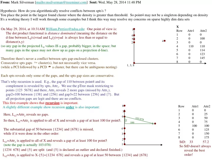
X Row Attr1 Attr2 1 0 0 2 0 100 3 0 0 4 110 110 5 0 114 6 0 123 7 0 145 8 0 0 From: Mark Silverman [mailto:msilverman@treeminer.com] Sent: Wed, May 28, 2014 11:48 PM Hypothesis: How do you algorithmically resolve conflicts between spts's ? You place the point in the largest found cluster where the density is greater than threshold. So point4 may not be a singleton depending on density It's a working theory I will work through some examples but I think this way may resolve my concerns on sparse highly dim data sets 7 6 5 4 2 1, 3, 8 8 Row Attr1 Attr2 1 0 0 2 0 25 3 0 50 4 0 75 5 100 100 6 0 125 7 0 150 8 0 175 7 6 103.078 25 100 5 4 3 2 1 On May 29, 2014, at 10:31AMWilliam.Perrizo@ndsu.edu: One point of view is: The dot product functional is distance dominated (meaning the distance on the d-line between Ld(x)=xod and Ld(y)=yod is always less than or equal to distance(x,y) (so any gap in the projected Ld values IS a gap, probably bigger, in the space; but many gaps in the space may not show up as gaps on a projection d-line). Therefore there's never a conflict between spts gap-enclosed clusters. Consecutive spts gaps cluster(s), but not necessarily vice versa. (while a PCI followed by a PCD a cluster, but there can be ambiguous nesting) Each spts reveals only some of the gaps, and the spts gap sizes are conservative. That’s why recursion is used. E.g., the gap of 110 between point4 and its complement is revealed by spts, Attr1. We use the pTree mask restricting to points {123 5678} and there, Attr2 reveals 2 more gaps (missed by Attr1), gap2=100 between {138} and {256} and gap3=22 between {256} and {7}. But all projection gaps are legit and there are no conflicts. This first example shows that recursion is important. A slightly different example show recursion order is also important: Here, Le2=Attr2 reveals no gaps. So then, Le1=Attr1 is applied to all of X and reveals a gap of at least 100 for point5. The substantial gap of 50 between {1234} and {678} is missed, while if it were done in the other order: Le1=Attr1 is applied to all of X and reveals a gap of at least 100 for point5 (note the gap is actually 103.078) StD: 33 57.2 So StD doesn't always reveal the best order! {1234 678} and {5} are split (and {5} is declared an outlier and declared finished.) Le2=Attr2 is applied to X-{5}={1234 678} and reveals a gap of at least 50 between {1234} and {678}
Frommsilverman@treeminer.comSent Thur, May 29, 2014 12:21 I see the confusion. You start with any spts then recurse thru unclustered pts. {recurse on each subcluster set produced by that SPTS}. I'm thinking how to do this in hadoop in parallel - I have different spts arriving at different processors, so my issue is what happens if these processors arrive at different conclusions. Good question! Possible answer: Parallelize incrementally (as the recursion progresses). Let's assume the entire dataset is replicated to all nodes. ( If not, modifications need to be made.) Do the first dot product spts splitting. We get a mask pTree for each gap-enclosed sub-cluster (a mask pTree in Hadoop, is a horizontal array of bits specifying which documents are in the sub-cluster) In parallel, send each of those mask pTrees to a different node. (also send all of those mask pTrees to the designated “dendogram building” node). Second issue is that entire dataset cannot fit into memory so getting to density is a challenge. If we deal strictly with gaps, density may not be necessary. In any case, Barrel Density could give a good approx. Once the Linear distrib is done, compute the distribution of radial reach distances from the d-line. The max (or last PCD) of those numbers should give you a good barrel radius. From here one could simply take the max of the max radial reach (mrr) and the linear projection radius (lpr) as a radius, r. The volume would be roughly rn to divided into the count for density. If that proves to rough, the actual barrel volume is roughly mrrn-1 * lpr From: Mark Silverman Sent: Thursday, May 29, 2014 1:09 Each processor sees only some of attributes, not all. I'm thinking we have one pass through the attributes to get stats and also we can pull radius. Then we can sequentially process Only issue now is cluster merge which I don't see a way around but huge benefit if we can figure it out which we will :) Sparseness is a major issue-for example in a million docs the word "arrrgghhh" in a single document could cluster. We might want it to be an outlier (2 emails with “arrrgghhh” probably came from the same sender?). Or we might make a pass through our vocab, flagging those words that we don't want to trigger a cut. Then we would not use those columns as spts's. Clearly we need to apply some sort of relevance tuning probably better than stddev. Agree. Previous slide, last example shows that stddev can fail. Sparseness breaks kmeans because the average of any attribute will tend to be pretty close to zero. So I'm trying to keep that in mind. The other issue is that we cannot have a single processor manage every attribute so we need this notion of merging clusters somehow - that's why I've been thinking about the issue where two processors make two different decisions. I have to think about that more. We could think about those decisions as being separate collections of mask pTrees, then we just AND the collections for the combined dendogram level? Consider also steaming data where later arriving data may need to be either placed in an existing cluster or a new one. I think it's the same problem? We should always save the spts cut_points and use those to put new data in the proper cluster. If new data pt, y, is in the middle of a previous gap, it is the start of a new cluster? We could just build dis2(X,y) and calculate the minimum to decide.I’m going to assume: 1. Gap-based clustering (or splitting) will suffice in text mining (no need to split at PCCs also). Gap-based never requires a dendogram and therefore never requires density nor fusion. When I use the term “gap” I will mean gap > Gap_Threshold for some chosen GT. 2. The initial dispersal of attributes to nodes is a partition (mutually exclusive). Then for d, to get “X dot d” spts use a master-slave (slaves compute their parts and send their partial spts to the master to be added onto the final spts Of course, if d=ek the spts is the just the given kth column and is available without any required computation at one node. Thought: A cluster subset is always expressed as a mask pTree (a row of bits in Hadoop). Those results can be sent to a master node to build the full clustering (by ANDind each pair coming from different sites). I think such a master could keep up with the slaves working in parallel. We just have to AND all pairs of mask pTrees, one coming from each of two different sites. The result is one clustering of the entire dataset (the one our gap-based FAUST Oblique algorithm produces for the chosen Minimum Gap Threshold). In the text mining case I am going to guess using only the ek’s will suffice (We won’t even need combo of them). Said another way: A gap in any “X dot d” spts gives us two disjoint mask pTrees that split the space in two and we know that no bonafide cluster subset can span that divide (so there should never be a need to fuse). Therefore it doesn’t matter where cluster subsets (or splits) are revealed – at one site or by ANDing pairs of mask pTrees from different sites. From this point of view, a merge step may be unnecessary. Disclaimer: In order to be guaranteed we have gotten all linear gaps, we may need to employ all unit vectors, d (a full partitioning of the unit n-1_half_sphere). And there are gaps that are not linear (not hyperplanar).
Machine Learning = moving data up some concept hierarchy (increasing information and/or/by reducing volume). ML takes two forms: clustering and classification (unsupervised and supervised). Clustering groups similar objects into a single higher level object or a cluster. Classification does the same but is supervised by an existing class assignment function on a Training Set, f:TS{Classes}. 1. Clustering can be done for Anomaly Detection (detecting those object that are dissimilar from the rest; which boils down to finding singleton [and/or doubleton..] clusters. 2. Clustering can be done to develop a Training Set for classification of future unclassified objects. Machine Learning moves data up a concept hierarchy, according to some criteria which we call a similarity. A similarity is usually a function, s:XXCardinalSet s.t. xX s(x,x)s(x,y) yX (every x must be at least as similar to itself as it is to any other object) and s(x,y)=s(y,x). OrdinalSet is usually a subset of {0,1,...} (e.g., binary {0,1}={No,Yes}). Classification is binary clustering: s(x,y)=1 iff f(x)=f(y). Using that part of f which is known to predict that which is unknown NCL: (k is discovered, not specified. Assign each (object,class) a ClassWeight, CWReals (could be <0). Classes "take next ticket" as they're discovered (tickets are 1,2,... Initially, all classes empty; All CWs=0. Do for next d, compute Ld = Xod until after masking off new cluster, count is too high (doesn't drop enough) For the next PCI in Ld (next-larger starting from smallest) If followed by a PCD, declare next Classk and define it to be the set spherically gapped (or PCDed) around centroid, Ck=Avg or VoMk over Ld-1[PCI, PCD]. Mask off this ticketed new Classk and contin If followed by a PCI, declare next Classk and define it to be the set spherically gapped (or PCDed) around the centroid, Ck=Avg or VoMk over Ld-1[ (3PCI1+PCI2)/4, PCI2 ) Mask off this ticketed new Classk and continue. For the next-smaller PCI (starting from largest) in Ld If preceded by a PCD, declare next Classk and define it to be the set spherically gapped (or PCDed) around centroid Ck=Avg or VoMk over Ld-1[PCD, PCI]. Mask off this ticketed new Classk, contin. If preceded by a PCI, declare next Classk and define it to be the set spherically gapped (or PCDed) around the centroid, Ck=Avg or VoMk over Ld-1( PCI2, (3PCI1+PCI2)/4] Mask off this ticketed new Classk and continue.
Pillar pk-means clusterer (k is not specified - it reveals itself.) 1a. Choose m1 maximizing D1=Dis(X,avgX). 1b. Check if m1 is outlier with Sm1 1c. Repeat until m1 is a non-outlier 2a. Choose m2 maximizing D2=Dis(X,m1) 2b. Check if m2 is outlier with Sm2 2c. Repeat until m2 is a non-outlier. 2d. Compute M1,2=Pm1m2 M2,1=Pm1<m2 3a. Choose m3 maximizing D3=D2+Dis(X,m2) 3b. Check if m3 is outlier with Sm3 3c. Repeat until m3 is a non-outlier. 3d. Compute Mi,3=Pmim3 M3,i=Pmi<m3 i<3 4a. Choose m4 maximizing D4=D3+Dis(X,m3) 4b. Check if m4 is outlier with Sm4 4c. Repeat until m4 is a non-outlier. 4d. Compute Mi,4=Pmim4 M3,i=Pmi<m4 i<4 ... Do until the MinDist(mh,mk)k<h < Threshold Mj = &hj Mj,h are the mask pTrees of the k clusters for the k first round clusters. Apply pk-means from here on. m1 m4 m3 m2
x (x-p)o(x-p) - (x-p)od2 (x-p)o(x-p) d (x-p)od = |x-p| cos FAUST Oblique Analytics X(X1..Xn)Rn, |X|=N; Classes={C1..CK}; d=(d1..dn), |d|=1; p=(p1..pn)Rn; Functionals: p (X-p)o(X-p) - [(X-p)od]2 = XoX+pop-2Xop - [Xod-pod]2 XoX+pop-2Xop - Xod2 - 2pod Xod + pod2 XoX+pop-2Xop - Xod2 - 2pod Xod + pod2+XoX+pop or XoX+pop-2Xop - 2pod Xod + pod2 - Xod2 + XoX Ld,p (X-p)od= Xod-pod= Ld-pod Lmind,p,k= min(Ld,p&Ck) Lmaxd,p,k= max(Ld,p&Ck) Sp (X-p)o(X-p)= XoX+Xo(-2p)+pop Sminp,k = min(Sp&Ck) Smaxp,k = max(Sp&Ck) Rd,p Sp-L2d,p= XoX+Xo(-2p)+pop-L2d-2pod*Xod+pod2= L-2p-(2pod)d+pop+pod2+XoX-L2d Rmind,pd,k = min(Rd,p&Ck) Rmaxaxd,pd,k = max(Rd,p&Ck) FAUST CountChange clustererIf DensThres unrealized, cut C at PCCsLd,p&C with next (d,pd)dpSet FAUST TopKOutliersUse D2NN=SqDist(x, X')=rank2Sx for TopKOutlier-slider. FAUST Linear classifier yCk iff yLHk {z | Lmind,p,k (z-p)od Lmmaxd,pd,k} (d,p)dpSet LHk is a hull around Ck. dpSet is a set of (d,p) pairs, e.g., (Diag,DiagStartPt). RkiPtr(x,PtrRankiSx). RkiSD(x,rankiS2) ordered desc on rankiSx as constructed. Pre-compute what? 1. col stats(min, avg, max, std,...) ; 2. XoX; Xop, p=class_Avg/Med); 3. Xod, d=interclass_Avg/Med_UnitVector; 4. Xox, d2(X,x), Rkid2(X,x), xX, i=2..; 5. Ld,p and Rd,p d,pdpSet FAUST LinearSphericalRadial classifier yCk iff yLSRHk{z | Tmind,p,k (z-p)od Tmaxd,p,k (d,p)dpSet, T=L|S|R }
FAUST Oblique LSR Classification IRIS150 16 34 246 26 32 12 48 0 50 15 34 50 28 22 16 34 21 1 21 29 4746 153 6 0 99 393 1096 1217 1826 4954 482422 11 8134 9809 0 66 310 35246 12 1750 4104 270 792 26 5 1558 2568 0 55 3139 3850 Ld d=1000 p=origin S43 59 E 49 71 I 49 80 Ld d=0010 p=origin S 10 19 E 30 51 I 18 69 Ld d=0001 p=origin S 1 6 E 10 18 I 14 26 Ld d=0100 p=origin S 23 44 E 20 34.1 I 22 38 3000 331547 14 6120 6251 p=AvgS 50 34 15 2 0 279 5 171 186 748 998 1 517, 4 79 633 2.8 1633 14 158 199 5 3617 7 152 611 3 5813 21 234 793 110321 3 1417 712 636 9, 3 983 1369 p=AvgE 59 28 43 13 24 126 2 1 132 730 1622 2281 0 342610 388 1369 5.9 1146 14 319 453 0 2522 12 454 1397 5 36 47 23 1403 929 1892 2824 96 273 1776 2747 p=AvgI 66 30 55 20
o=origin; pRn; dRn, |d|=1; {Ck}k=1..K are the classes; An operation enclosed in a parallelogram, , means it is a pTree op, not a scalar operation (on just numeric operands) Lp,d (X - p) o d = Lo,d - [pod] minLp,d,k = min[Lp,d & Ck] maxLp,d,k = max[Lp,d & Ck[ = [minLo,d,k]- pod = [maxLo,d,k] - pod = min(Xod & Ck)- pod = max(Xod & Ck) - podOR = min(X&Ck) o d- pod = max(X&Ck) o d - pod Sp = (X - p)o(X - p) = -2Xop+So+pop = Lo,-2p + (So+pop) minSp,k=minSp&Ck maxSp,k = maxSp&Ck = min[(X o (-2p) &Ck)]+ (XoX+pop) =max[(X o (-2p) &Ck)] + (XoX+pop) OR= min[(X&Ck)o-2p]+ (XoX+pop) =max[(X&Ck)o-2p] + (XoX+pop) Rp,d Sp, - Lp,d2 minRp,d,k=min[Rp,d&Ck] maxRp,d,k=max[Rp,d&Ck] APPENDIX LSR IRIS150-. Consider all 3 functionals, L, S and R. What's the most efficient way to calculate all 3?\ I suggest that we use each of the functionals with each of the pairs, (p,d) that we select for application (since, to get R we need to compute L and S anyway). So it would make sense to develop an optimal (minimum work and time) procedure to create L, S and R for any (p,d) in the set.
C13 C8,1: D=0110 Ch,1: D=10-10 Ca,1: D=0011 Cg,1: D=1-100 Cf,1: D=1111 Ce,1: D=0111 C5,1: D=1100 C6,1: D=1010 C9,1: D=0101 C7,1: D=1001 C2,3: D=0100 Cb,1: D=1110 C3,3: D=0010 Cc,1: D=1101 C4,1: D=0001 Cd,1: D=1011 C1,1: D=1000 55 169 y isa O if yoD(-,55)(169,) L H y isa O|S if yoD Ce,1 [55,169] 81 182 y isa O if yoD(-,81)(182,) L H y isa O|S if yoD Cc,1 [81,182] 68 117 y isa O if yoD(-,68)(117,) L H y isa O|S if yoD C6,1 [68,117] 3 46 y isa O if yoD(-,3)(46,) L H y isa O|S if yoD Ci,1 [3,46] 10 22 y isa O if yoD(-,10)(22,) L H y isa O|S if yoD Ch,1 [10,22] 84 204 y isa O if yoD(-,84)(204,) L H y isa O|S if yoD Cg,1 [84,204] 39 127 y isa O if yoD(-,39)(127,) L H y isa O|S if yoD Cf,1 [39,127] 71 137 y isa O if yoD(-,71)(137,) L H y isa O|S if yoD Cd,1 [71,137] 10 19 y isa O if yoD(-,10)(19,) L H y isa O|S if yoD C4,1 [10,19] 1 6 y isa O if yoD(-,1)(6,) L H y isa O|S if yoD C5,1 [1,6] 23 44 y isa O if yoD(-,23)(44,) L H y isa O|S if yoD C3,3 [23,44] 54 146 y isa O if yoD(-,54)(146,) L H y isa O|S if yoD C7,1 [54,146] 12 91 y isa O if yoD(-,12)(91,) L H y isa O|S if yoD Cb,1 [12,91] 26 61 y isa O if yoD(-,26)(61,) L H y isa O|S if yoD Ca,1 [26,61] 36 105 y isa O if yoD(-,36)(105,) L H y isa O|S if yoD C9,1 [36,105] 44 100 y isa O if yoD(-,44)(100,) L H y isa O|S if yoD C8,1 [44,100] 43 58 y isa O if yoD(-,43)(58,) L H y isa O|S if yoD C2,3 [43,58] 400 1000 1500 2000 2500 3000 LSR on IRIS150 y isa OTHER if yoDse (-,495)(802,1061)(2725,) Dse 9 -6 27 10 495 802 S 1270 2010 E 1061 2725 I L H y isa OTHER or S if yoDse C1,1 [ 495 , 802] y isa OTHER or I if yoDse C1,2 [1061 ,1270] y isa OTHER or E or I if yoDse C1,3 [1270 ,2010 C1,3: 0 s 49 e 11 i y isa OTHER or I if yoDse C1,4 [2010 ,2725] Dei -3 -2 3 3 -117 -44 E y isa O if yoDei (-,-117)(-3,) -62 -3 I y isa O or E or I if yoDei C2,1 [-62 ,-44] L H y isa O or I if yoDei C2,2 [-44 , -3] C2,1: 2 e 4 i Dei 6 -2 3 1 420 459 E y isa O if yoDei (-,420)(459,480)(501,) 480 501 I y isa O or E if yoDei C3,1 [420 ,459] L H y isa O or I if yoDei C3,2 [480 ,501] Continue this on clusters with OTHER + one class, so the hull fits tightely (reducing false positives), using diagonals? The amount of work yet to be done., even for only 4 attributes, is immense.. For each D, we should fit boundaries for each class, not just one class. For 4 attributes, I count 77 diagonals*3 classes = 231 cases. How many in the Enron email case with 10,000 columns? Too many for sure!! D, not only cut at minCoD, maxCoD but also limit the radial reach for each class (barrel analytics)? Note, limiting the radial reach limits all other directions [other than the D direction] in one step and therefore by the same amount. I.e., it limits all directions assuming perfectly round clusters). Think about Enron, some words (columns) have high count and others have low count. Our radial reach threshold would be based on the highest count and therefore admit many false positives. We can cluster directions (words) by count and limit radial reach differently for different clusters??
Dot Product SPTS computation:XoD = k=1..nXkDk D2,0 D2,1 D1,0 D1,1 D X1*X2 = (21 p1,1 +20 p1,0) (21 p2,1 +20 p2,0) = 22 p1,1 p2,1 +21( p1,1 p2,0+ p2,1 p1,0) + 20 p1,0 p2,0 1 1 3 3 1 1 pXoD,1 pXoD,0 pXoD,3 pXoD,2 X X1 X2 p11 p10 p21 p20 XoD 0 1 1 0 1 0 0 1 1 1 1 1 1 1 0 1 1 1 0 1 0 1 1 0 1 0 0 1 0 0 6 9 9 0 1 1 0 1 1 1 3 2 1 0 1 0 1 1 1 1 0 0 0 0 1 0 1 & & & & 0 1 1 0 1 1 1 1 0 1 1 0 1 0 1 1 0 1 0 1 1 0 1 0 pX1*X2,0 0 1 0 pX1*X2,1 0 1 0 0 1 0 X X1 X2 pX1*X2,2 pX1*X2,3 p11 p10 p21 p20 X1*X2 D2,0 D2,1 D1,0 D1,1 D ( ( = 22 = 22 1 p1,1 1 p1,1 + 1 p2,1 ) + 1 p2,1 ) + 1 p2,0 ) + 1 p2,0 ) + 21 (1 p1,0 + 21 (1 p1,0 + 1 p11 + 1 p11 + 20 (1 p1,0 + 20 (1 p1,0 + 1 p2,0 + 1 p2,0 + 1 p2,1 ) + 1 p2,1 ) 1 3 2 1 3 1 0 1 1 1 1 0 0 1 0 1 1 1 1 9 2 1 1 0 0 0 0 0 1 0 1 0 1 1 0 3 3 1 1 & & 0 1 0 0 0 0 0 0 1 CAR12,3 1 1 0 0 1 0 0 0 1 0 1 0 1 0 1 CAR11,2 0 0 0 1 0 0 CAR10,1 CAR22,3 & pX1*X2,1 pX1*X2,2 pX1*X2,3 pX1*X2,0 & & & CAR21,2 0 1 1 0 0 0 1 0 1 0 0 1 0 0 0 1 0 0 0 1 1 1 0 0 CAR13,4 PXoD,0 PXoD,3 PXoD,2 PXoD,1 0 1 0 0 0 0 1 0 1 0 1 0 1 1 0 PXoD,4 0 1 0 0 0 0 0 1 0 0 0 1 0 1 0 Different data. CAR10,1 pTrees XoD 0 0 1 X 0 0 0 1 0 1 0 0 1 0 1 0 0 0 0 1 1 0 0 1 1 1 1 0 0 1 1 0 1 1 1 0 0 0 1 1 0 1 0 1 1 0 1 1 0 1 1 1 0 0 1 1 1 1 0 1 0 0 1 0 1 0 0 1 1 0 0 0 1 0 0 1 1 3 2 1 3 1 0 1 1 1 1 0 0 1 0 1 1 1 6 18 9 PXoD,0 PXoD,2 PXoD,1 PXoD,3 1 1 0 1 1 0 1 1 1 1 0 1 & & & & & & & & & & & & & & /*Calc PXoD,i after PXoD,i-1 CarrySet=CARi-1,i RawSet=RSi */ INPUT: CARi-1,i, RSi ROUTINE: PXoD,i=RSiCARi-1,i CARi,i+1=RSi&CARi-1,i OUTPUT: PXoD,i, CARi,i+1 1 1 0 0 1 1 0 1 1 1 0 1 1 1 0 0 1 1 0 1 1 0 1 0 1 1 1 0 1 0 We have extended the Galois field, GF(2)={0,1}, XOR=add, AND=mult to pTrees. SPTS multiplication: (Note, pTree multiplication = &)
Example: FAUST Oblique: XoD used in CCC, TKO, PLC and LARC) and (x-X)o(x-X) p1 p1 p1 p,0 p,0 p,0 p3 p3 p3 p2 p2 p2 X X1 X2 p11 p10 p21 p20 XoD XoD XoD = -2Xox+xox+XoX is used in TKO. 0 0 0 0 1 1 1 0 0 1 0 1 1 1 0 1 1 1 3 9 2 2 3 3 3 6 5 0 1 0 0 0 0 0 0 0 1 0 1 1 1 0 0 1 1 1 3 2 1 0 1 0 1 1 1 1 0 0 0 0 1 0 1 n=1 p=2 n=0 p=2 P &p0 P=p0&P P p1 P=P&p1 D2,0 D2,0 D2,0 D2,1 D2,1 D2,1 D1,0 D1,0 D1,0 D1,1 D1,1 D1,1 D=x2 D=x1 D=x3 0 1 1 0 1 1 1 1 1 1 1 1 1 1 1 1 1 1 32 1*21+ 22 1*21+1*20=3 so -2x1oX = -6 0 1 0 1 0 0 2 1 1 1 3 0 0 1 1 1 1 0 n=3 p=2 n=2 p=1 n=1 p=1 n=0 p=1 P &p2 P=p'2&P P p3 P &p1 P &p0 P=P&p'3 P=p1&P P=p0&P RankN-1(XoD)=Rank2(XoD) 0 0 0 1 0 1 1 0 1 1 0 1 1 0 1 1 0 0 0 1 0 1 0 1 1 1 0 1 1 1 1 0 1 1 0 1 1<2 2-1=1 0*23+ 0<1 1-0=1 0*23+0*22 21 0*23+0*22+1*21+ 11 0*23+0*22+1*21+1*20=3 so -2x2oX= -6 RankN-1(XoD)=Rank2(XoD) n=2 p=2 n=1 p=2 n=0 p=1 P=p'1&P P &p1 P=P&p2 P=p0&P P p2 P &p0 0 0 1 1 1 0 0 1 1 0 1 1 1 0 1 1 1 1 0 0 1 0 1 1 0 0 1 22 1*22+ 1<2 2-1=1 1*22+0*21 11 1*22+0*21+1*20=5 so -2x3oX= -10 So in FAUST, we need to construct lots of SPTSs of the type, X dotted with a fixed vector, a costly pTree calculation (Note that XoX is costly too, but it is a 1-time calculation (a pre-calculation?). xox is calculated for each individual x but it's a scalar calculation and just a read-off of a row of XoX, once XoX is calculated.. Thus, we should optimize the living he__ out of the XoD calculation!!! The methods on the previous seem efficient. Is there a better method? Then for TKO we need to computer ranks: RankK: p is what's left of K yet to be counted, initially p=K V is the RankKvalue, initially 0. For i=bitwidth+1 to 0 if Count(P&Pi) p { KVal=KVal+2i; P=P&Pi}; else /* < p */ { p=p-Count(P&Pi);P=P&P'i }; RankN-1(XoD)=Rank2(XoD)
pTree Rank(K) computation: (Rank(N-1) gives 2nd smallest which is very useful in outlier analysis?) p1 p,0 p3 p2 X X1 X2 p11 p10 p21 p20 XoD 1 0 0 1 1 1 2 3 3 0 0 0 0 1 1 1 3 2 1 0 1 0 1 1 1 1 0 0 0 0 1 0 1 D2,0 D2,1 D1,0 D1,1 D 0 1 3 3 0 1 RankKval= 0 1 0 0 0 0 0 23 * + 22 * + 21 * + 20 * = 5P=MapRankKPts= ListRankKPts={2} RankN-1(XoD)=Rank2(XoD) n=3 p=2 n=2 p=2 n=1 p=2 n=0 p=2 P &p2 P p3 P &p1 P &p0 1 0 0 0 1 1 0 1 1 1 0 0 0 1 1 1 1 1 0 1 1 0 1 1 22 1*23+ 0<2 2-0=2 1*23+0*22+ 0<2 2-0=2 1*23+0*22+0*21+ 22 1*23+0*22+0*21+1*20=9 0 1 1 0 1 1 0 1 1 0 1 1 P=P&p3 P=p'2&P P=p'1&P P=p0&P Cross out the 0-positions of P each step. (n=3) c=Count(P&P4,3)= 3 < 6 p=6–3=3; P=P&P’4,3 masks off highest 3 (val 8) {0} X P4,3P4,2P4,1 P4,0 0 1 1 1 0 0 0 0 1 0 1 1 1 1 10 5 6 7 11 9 3 1 0 0 0 1 1 0 1 0 1 1 1 0 1 (n=2) c=Count(P&P4,2)= 3 >= 3 P=P&P4,2 masks off lowest 1 (val 4) {1} (n=1) c=Count(P&P4,1)=2 < 3 p=3-2=1; P=P&P'4,1 masks off highest 2 (val8-2=6 ) {0} {1} (n=0) c=Count(P&P4,0 )=1 >= 1 P=P&P4,0 RankKval=0; p=K; c=0; P=Pure1; /*Note: n=bitwidth-1. The RankK Points are returned as the resulting pTree, P*/ For i=n to 0 {c=Count(P&Pi); If (c>=p) {RankVal=RankVal+2i; P=P&Pi}; else {p=p-c;P=P&P'i }; return RankKval, P; /* Above K=7-1=6 (looking for the Rank6 or 6th highest vaue (which is also the 2nd lowest value) */ {0} {1} {0} {1}
applied to S, a column of numbers in bistlice format (an SpTS), will produce the DistributionTree of S DT(S) depth=h=0 15 p6' 1 1 1 1 1 0 0 0 0 0 0 0 0 0 0 5/64 [0,64) p6' 1 1 1 1 1 0 0 0 0 0 0 0 0 0 0 p6' 1 1 1 1 1 0 0 0 0 0 0 0 0 0 0 p6' 1 1 1 1 1 0 0 0 0 0 0 0 0 0 0 p6' 1 1 1 1 1 0 0 0 0 0 0 0 0 0 0 p5' 1 1 1 0 0 1 0 0 0 0 0 0 0 0 1 p5' 1 1 1 0 0 1 0 0 0 0 0 0 0 0 1 p5' 1 1 1 0 0 1 0 0 0 0 0 0 0 0 1 2/32[64,96) p4' 1 0 0 1 0 0 0 0 0 0 1 0 1 0 0 1[32,48) p5' 1 1 1 0 0 1 0 0 0 0 0 0 0 0 1 3/32[0,32) p4' 1 0 0 1 0 0 0 0 0 0 1 0 1 0 0 2[96,112) p4' 1 0 0 1 0 0 0 0 0 0 1 0 1 0 0 0[64,80) p4' 1 0 0 1 0 0 0 0 0 0 1 0 1 0 0 1/16[0,16) p5' 1 1 1 0 0 1 0 0 0 0 0 0 0 0 1 p4' 1 0 0 1 0 0 0 0 0 0 1 0 1 0 0 p5' 1 1 1 0 0 1 0 0 0 0 0 0 0 0 1 p4' 1 0 0 1 0 0 0 0 0 0 1 0 1 0 0 p5' 1 1 1 0 0 1 0 0 0 0 0 0 0 0 1 p6' 1 1 1 1 1 0 0 0 0 0 0 0 0 0 0 p4' 1 0 0 1 0 0 0 0 0 0 1 0 1 0 0 p6' 1 1 1 1 1 0 0 0 0 0 0 0 0 0 0 p4' 1 0 0 1 0 0 0 0 0 0 1 0 1 0 0 p5' 1 1 1 0 0 1 0 0 0 0 0 0 0 0 1 p6' 1 1 1 1 1 0 0 0 0 0 0 0 0 0 0 p4 0 1 1 0 1 1 1 1 1 1 0 1 0 1 1 6[112,128) p4 0 1 1 0 1 1 1 1 1 1 0 1 0 1 1 1[48,64) p3' 0 0 1 1 1 1 1 1 0 1 0 0 0 0 1 1[16,24) p4 0 1 1 0 1 1 1 1 1 1 0 1 0 1 1 2/16[16,32) p4 0 1 1 0 1 1 1 1 1 1 0 1 0 1 1 2[80,96) p4 0 1 1 0 1 1 1 1 1 1 0 1 0 1 1 p4 0 1 1 0 1 1 1 1 1 1 0 1 0 1 1 p4 0 1 1 0 1 1 1 1 1 1 0 1 0 1 1 p4 0 1 1 0 1 1 1 1 1 1 0 1 0 1 1 p5 0 0 0 1 1 0 1 1 1 1 1 1 1 1 0 p5 0 0 0 1 1 0 1 1 1 1 1 1 1 1 0 2/32[32,64) p5 0 0 0 1 1 0 1 1 1 1 1 1 1 1 0 p5 0 0 0 1 1 0 1 1 1 1 1 1 1 1 0 ¼[96,128) p5 0 0 0 1 1 0 1 1 1 1 1 1 1 1 0 p5 0 0 0 1 1 0 1 1 1 1 1 1 1 1 0 p5 0 0 0 1 1 0 1 1 1 1 1 1 1 1 0 p5 0 0 0 1 1 0 1 1 1 1 1 1 1 1 0 p3' 0 0 1 1 1 1 1 1 0 1 0 0 0 0 1 1[48,56) p3 1 1 0 0 0 0 0 0 1 0 1 1 1 1 0 1[24,32) p3 1 1 0 0 0 0 0 0 1 0 1 1 1 1 0 0[56,64) p3' 0 0 1 1 1 1 1 1 0 1 0 0 0 0 1 0[0,8) p3' 0 0 1 1 1 1 1 1 0 1 0 0 0 0 1 1[32,40) p3 1 1 0 0 0 0 0 0 1 0 1 1 1 1 0 1[8,16) p3 1 1 0 0 0 0 0 0 1 0 1 1 1 1 0 0[40,48) p6 0 0 0 0 0 1 1 1 1 1 1 1 1 1 1 10/64 [64,128) p6 0 0 0 0 0 1 1 1 1 1 1 1 1 1 1 p3' 0 0 1 1 1 1 1 1 0 1 0 0 0 0 1 2[80,88) p3' 0 0 1 1 1 1 1 1 0 1 0 0 0 0 1 3[112,120) p6 0 0 0 0 0 1 1 1 1 1 1 1 1 1 1 p6 0 0 0 0 0 1 1 1 1 1 1 1 1 1 1 p6 0 0 0 0 0 1 1 1 1 1 1 1 1 1 1 p6 0 0 0 0 0 1 1 1 1 1 1 1 1 1 1 p6 0 0 0 0 0 1 1 1 1 1 1 1 1 1 1 p6 0 0 0 0 0 1 1 1 1 1 1 1 1 1 1 p3 1 1 0 0 0 0 0 0 1 0 1 1 1 1 0 0[88,96) p3 1 1 0 0 0 0 0 0 1 0 1 1 1 1 0 3[120,128) p3' 0 0 1 1 1 1 1 1 0 1 0 0 0 0 1 p3' 0 0 1 1 1 1 1 1 0 1 0 0 0 0 1 0[96,104) p3 1 1 0 0 0 0 0 0 1 0 1 1 1 1 0 p3 1 1 0 0 0 0 0 0 1 0 1 1 1 1 0 2[194,112) UDR Univariate Distribution Revealer (on Spaeth:) 5 10 depth=h=1 node2,3 [96.128) yofM 11 27 23 34 53 80 118 114 125 114 110 121 109 125 83 p6 0 0 0 0 0 1 1 1 1 1 1 1 1 1 1 p5 0 0 0 1 1 0 1 1 1 1 1 1 1 1 0 p4 0 1 1 0 1 1 1 1 1 1 0 1 0 1 1 p3 1 1 0 0 0 0 0 0 1 0 1 1 1 1 0 p2 0 0 1 0 1 0 1 0 1 0 1 0 1 1 0 p1 1 1 1 1 0 0 1 1 0 1 1 0 0 0 1 p0 1 1 1 0 1 0 0 0 1 0 0 1 1 1 1 p6' 1 1 1 1 1 0 0 0 0 0 0 0 0 0 0 p5' 1 1 1 0 0 1 0 0 0 0 0 0 0 0 1 p4' 1 0 0 1 0 0 0 0 0 0 1 0 1 0 0 p3' 0 0 1 1 1 1 1 1 0 1 0 0 0 0 1 p2' 1 1 0 1 0 1 0 1 0 1 0 1 0 0 1 p1' 0 0 0 0 1 1 0 0 1 0 0 1 1 1 0 p0' 0 0 0 1 0 1 1 1 0 1 1 0 0 0 0 Y y1 y2 y1 1 1 y2 3 1 y3 2 2 y4 3 3 y5 6 2 y6 9 3 y7 15 1 y8 14 2 y9 15 3 ya 13 4 pb 10 9 yc 11 10 yd 9 11 ye 11 11 yf 7 8 3 2 2 8 f= 1 2 1 1 0 2 2 6 0 1 1 1 1 0 1 000 2 0 0 2 3 3 depthDT(S)b≡BitWidth(S) h=depth of a node k=node offset Nodeh,k has a ptr to pTree{xS | F(x)[k2b-h+1, (k+1)2b-h+1)} and its 1count Pre-compute and enter into the ToC, all DT(Yk) plus those for selected Linear Functionals (e.g., d=main diagonals, ModeVector . Suggestion: In our pTree-base, every pTree (basic, mask,...) should be referenced in ToC( pTree, pTreeLocationPointer, pTreeOneCount ).and these OneCts should be repeated everywhere (e.g., in every DT). The reason is that these OneCts help us in selecting the pertinent pTrees to access - and in fact are often all we need to know about the pTree to get the answers we are after.).
D2,0 D2,1 D1,0 D1,1 D So let us look at ways of doing the work to calculate As we recall from the below, the task is to ADD bitslices giving a result bitslice and a set of carry bitslices to carry forward XoD = k=1..nXk*Dk 1 1 3 3 1 1 ( ( = 22 = 22 1 p1,1 1 p1,1 + 1 p2,1 ) + 1 p2,1 ) ( ( ( ( + 1 p2,0 ) + 1 p2,0 ) 1 p1,0 1 p1,0 + 1 p11 + 1 p11 1 p1,0 1 p1,0 + 21 + 21 + 1 p2,0 + 1 p2,0 + 1 p2,1 ) + 1 p2,1 ) + 20 + 20 pTrees XoD X 1 0 0 1 0 0 0 1 1 0 1 1 1 3 2 1 0 1 0 1 1 1 1 0 0 0 0 1 0 1 6 9 9 0 1 1 0 1 1 1 1 0 1 1 0 1 0 1 1 0 1 0 1 1 1 1 1 1 0 0 I believe we add by successive XORs and the carry set is the raw set with one 1-bit turned off iff the sum at that bit is a 1-bit Or we can characterize the carry as the raw set minus the result (always carry forward a set of pTrees plus one negative one). We want a routine that constructs the result pTree from a positive set of pTrees plus a negative set always consisting of 1 pTree. The routine is: successive XORs across the positive set then XOR with the negative set pTree (because the successive pset XOR gives us the odd values and if you subtract one pTree, the 1-bits of it change odd to even and vice versa.): /*For PXoD,i (after PXoD,i-1). CarrySetPos=CSPi-1,i CarrySetNeg=CSNi-1,i RawSet=RSi CSP-1=CSN-1=*/ INPUT: CSPi-1, CSNi-1, RSi ROUTINE: PXoD,i=RSiCSPi-1,iCSNi-1,i CSNi,i+1=CSNi-1,iPXoD,i; CSPi,i+1=CSPi-1,iRSi-1; OUTPUT: PXoD,i, CSNi,i+1 CSPi,i+1 0 1 1 0 1 1 1 1 0 0 0 0 1 0 1 1 1 0 1 0 1 CSN-1.0PXoD,0 CSP-1,0RS0 RS1 CSN0,1= CSP0,1= CSP-1,0=CSN-1,0= RS0 PXoD,0 PXoD,1 1 1 0 1 0 1 0 1 1 1 1 0 0 1 1 0 1 1 1 0 1 0 0 0 1 1 0 1 0 1 = = 1 0 1 0 0 0 0 1 1 1 0 1 0 0 0
D2,0 D2,0 D2,1 D2,1 D1,0 D1,0 D1,1 D1,1 D D XoD = k=1..nXk*Dk 1 1 1 0 3 3 1 2 1 1 0 1 k=1..n ( = 22B Dk,B pk,B k=1..n ( Dk,B pk,B-1 + Dk,B-1 pk,B + 22B-1 k=1..n ( Dk,B pk,B-2 + Dk,B-1 pk,B-1 + Dk,B-2 pk,B + 22B-2 Xk*Dk = Dkb2bpk,b XoD=k=1,2Xk*Dk with pTrees: qN..q0, N=22B+roof(log2n)+2B+1 k=1..n ( +Dk,B-3 pk,B Dk,B pk,B-3 + Dk,B-1 pk,B-2 + Dk,B-2 pk,B-1 + 22B-3 = Dk(2Bpk,B +..+20pk,0) = (2BDk,B+..+20Dk,0) (2Bpk,B +..+20pk,0) . . . k=1..2 ( = 2BDkpk,B +..+ 20Dkpk,0 = 22 Dk,1 pk,1 k=1..n ( Dk,Bpk,B) = 22B( +Dk,Bpk,B-1) + 22B-1(Dk,B-1pk,B Dk,B pk,0 + Dk,2 pk,1 + Dk,1 pk,2 +Dk,0 pk,3 + 23 +..+20Dk,0pk,0 k=1..2 ( Dk,1 pk,0 + Dk,0 pk,1 + 21 pTrees k=1..n ( X Dk,2 pk,0 + Dk,1 pk,1 + Dk,0 pk,2 + 22 B=1 1 3 2 1 0 1 0 1 1 1 1 0 0 0 0 1 0 1 k=1..2 ( k=1..n ( Dk,0 pk,0 Dk,1 pk,0 + Dk,0 pk,1 + 20 + 21 q0 = p1,0 = no carry 1 1 0 k=1..n ( Dk,0 pk,0 + 20 ( ( = 22 = 22 1 p1,1 D1,1p1,1 + 1 p2,1 ) + D2,1p2,1 ) ( ( ( ( + 1 p2,0 ) + D2,0p2,0) D1,1p1,0 1 p1,0 + 1 p11 + D1,0p11 1 p1,0 D1,0p1,0 + 21 + 21 + 1 p2,0 + D2,1p2,0 + 1 p2,1 ) + D2,0p2,1) + 20 + 20 q1= carry1= 1 1 0 0 0 1 ( = 22 D1,1 p1,1 + D2,1 p2,1 ) ( ( + D2,0 p2,0) D1,1 p1,0 +D1,0 p11 D1,0 p1,0 + 21 + D2,1 p2,0 +D2,0 p2,1) + 20 0 0 0 q2=carry1= no carry 0 1 1 1 0 1 1 1 0 0 0 1 q0 = carry0= 0 1 1 1 0 0 0 1 1 0 1 1 1 1 0 0 0 0 1 1 0 1 0 1 1 0 1 1 1 1 2 1 1 q1=carry0+raw1= carry1= 1 1 1 1 1 1 q2=carry1+raw2= carry2= 1 1 1 q3=carry2 = carry3= A carryTree is a valueTree or vTree, as is the rawTree at each level (rawTree = valueTree before carry is incl.). In what form is it best to carry the carryTree over? (for speediest of processing?) 1. multiple pTrees added at next level? (since the pTrees at the next level are in that form and need to be added) 2. carryTree as a SPTS, s1? (next level rawTree=SPTS, s2, then s10& s20 = qnext_level and carrynext_level ? CCC ClustererIf DT (and/or DUT) not exceeded at C, partition C further by cutting at each gap and PCC in CoD For a table X(X1...Xn), the SPTS, Xk*Dk is the column of numbers, xk*Dk. XoD is the sum of those SPTSs, k=1..nXk*Dk So, DotProduct involves just multi-operand pTree addition. (no SPTSs and no multiplications) Engineering shortcut tricka would be huge!!!
Question: Which primitives are needed and how do we compute them? X(X1...Xn) D2NN yields a 1.a-type outlier detector (top k objects, x, dissimilarity from X-{x}). D2NN = each min[D2NN(x)] (x-X)o(x-X)= k=1..n(xk-Xk)(xk-Xk)=k=1..n(b=B..02bxk,b-2bpk,b)( (b=B..02bxk,b-2bpk,b) ----ak,b--- b=B..02b(xk,b-pk,b) ) ( 22Bak,Bak,B + =k=1..n( b=B..02b(xk,b-pk,b) )( 22B-1( ak,Bak,B-1 + ak,B-1ak,B ) + { 22Bak,Bak,B-1 } =k (2Bak,B+ 2B-1ak,B-1+..+ 21ak, 1+ 20ak, 0) (2Bak,B+ 2B-1ak,B-1+..+ 21ak, 1+ 20ak, 0) 22B-2( ak,Bak,B-2 + ak,B-1ak,B-1 + ak,B-2ak,B ) + {2B-1ak,Bak,B-2 + 22B-2ak,B-12 22B-3( ak,Bak,B-3 + ak,B-1ak,B-2 + ak,B-2ak,B-1 + ak,B-3ak,B ) + { 22B-2( ak,Bak,B-3 + ak,B-1ak,B-2 ) } 22B-4(ak,Bak,B-4+ak,B-1ak,B-3+ak,B-2ak,B-2+ak,B-3ak,B-1+ak,B-4ak,B)... {22B-3( ak,Bak,B-4+ak,B-1ak,B-3)+22B-4ak,B-22} =22B ( ak,B2 + ak,Bak,B-1 ) + 22B-1( ak,Bak,B-2 ) + 22B-2( ak,B-12 + ak,Bak,B-3 + ak,B-1ak,B-2 ) + 22B-3( ak,Bak,B-4+ak,B-1ak,B-3) + 22B-4ak,B-22 ... X(X1...Xn) RKN (Rank K Nbr), K=|X|-1, yields1.a_outlier_detector (top y dissimilarity from X-{x}). ANOTHER TRY! Install in RKN, each RankK(D2NN(x)) (1-time construct but for. e.g., 1 trillion xs? |X|=N=1T, slow. Parallelization?) xX, the square distance from x to its neighbors (near and far) is the column of number (vTree or SPTS) d2(x,X)= (x-X)o(x-X)= k=1..n|xk-Xk|2= k=1..n(xk-Xk)(xk-Xk)= k=1..n(xk2-2xkXk+Xk2) Should we pre-compute all pk,i*pk,j p'k,i*p'k,j pk,i*p'k,j D2NN=multi-op pTree adds? When xk,b=1, ak,b=p'k,b and when xk,b=0, ak,b= -pk.b So D2NN just multi-op pTree mults/adds/subtrs? Each D2NN row (each xX) is separate calc. = -2 kxkXk + kxk2 + kXk2 3. Pick this from XoX for each x and add to 2. = -2xoX + xox + XoX 5. Add 3 to this k=1..n i=B..0,j=B..02i+jpk,ipk,j 1. precompute pTree products within each k i,j 2i+j kpk,ipk,j 2. Calculate this sum one time (independent of the x) -2xoX cost is linear in |X|=N. xox cost is ~zero. XoX is 1-time -amortized over xX (i.e., =1/N) or precomputed The addition cost, -2xoX + xox + XoX, is linear in |X|=N So, overall, the cost is linear in |X|=n. Data parallelization? No! (Need all of X at each site.) Code parallelization? Yes! (After replicating X to all sites, Each site creates/saves D2NN for its partition of X, then sends requested number(s) (e.g., RKN(x) ) back.
LSR on IRIS150-3 Here we use the diagonals. d=e1 p=AVGs, L=(X-p)od 43 58 S 49 70 E 49 79I d=e4 p=AvgS, L=(X-p)od -2 4 S&L 7 16 E&L 11 23I&L d=e4 p=AvgS, L=(X-p)od -2 4 S&L 7 16 E&L 11 23I&L R(p,d,X) SEI 0 128 270 393 1558 3444 [43,49) S(16) 0 128 [49,58) E(24)I(6) 0 S(34) 99 393 1096 1217 1825 [70,79] I(12) 2081 3444 [58,70) E(26) I(32) 270 792 1558 2567 30ambigs, 5 errs -2,4) 50 -2,4) 50 [7,11) 28 [7,11) 28 [11,16) 22, 16 127.5 648.7 1554.7 2892 [11,16) 22, 16 5.7 36.2 151.06 611 [16,23] I=34 [16,23] I=34 E(50) I(7) 49 49 (36,7) 63 70 (11) d=e1 p=AS L=(X-p)od (-pod=-50.06) -7.06 7.94 S&L -1;06 19.94 E&L -1.06 28.94 I&L d=e1 p=AS L=(X-p)od (-pod=-50.06) -7.06 7.94 S&L -1;06 19.94 E&L -1.06 28.94 I&L d=e1 p=AS L=(X-p)od (-pod=-50.06) -7.06 7.94 S&L -1;06 19.94 E&L -1.06 28.94 I&L -8,-2 16 [-2,8) 34, 24, 6 0 99 393 1096 1217 1825 [8,20) 26, 32 270 792 1558 2567 [20,29] 12 E=22 I=7 p=AvgS E=22 I=8 p=AvgI E=17 I=7 p=AvgE E=26 I=5 p=AvgS -8,-2 16 -8,-2 16 [-2,8) 34, 24, 6 0 99 393 1096 1217 1825 [-2,8) 34, 24, 6 0 99 393 1096 1217 1825 [8,20) w p=AvgI 26, 32 0.62 34.9 387.8 1369 [8,20) w p=AvgE 26, 32 1.9 51.8 78.6 633 [20,29] 12 [20,29] 12 Only overlap L=[58,70), R[792,1557] (E(26),I(5)) With just d=e1, we get good hulls using LARC: While Ip,d containing >1class, for next (d,p) create L(p,d)Xod-pod, R(p,d)XoX+pop-2Xop-L2 1. MnCls(L), MxCls(L), create a linear boundary. 2. MnCls(R), MxCls(R).create a radial boundary. 3. Use R&Ck to create intra-Ck radial boundaries Hk = {I | Lp,d includes Ck} <--E=6 I=4 p=AvgE <--E=25 I=10 p=AvgI d=e4 p=AvgS, L=(X-p)od -2 4 S&L 7 16 E&L 11 23I&L [16,23] I=34 -2,4) 50 [7,11) 28 [11,16) 22, 16 127.5 1555 2892 Here we try using other p points for the R step (other than the one used for the L step). d=e1 p=AvgS, L=Xod 43 58 S&L 49 70 E&L 49 79 I&L R & L I(1) I(42) For e4, the best choice of p for the R step is also p=AvgE. (There are mistakes in this column on the previous slide!) There is a best choice of p for the R step (p=AvgE) but how would we decide that ahead of time?
SRR(AVGs,dse) on C1,1 0 154 S y isa O if yoD(-,43)(79,) d=e1=1000; The xod limits: 43 58 S 49 70 E 49 79 I y isa O or S( 9) if yoD[43,47] y isa O if yoD[43,47]&SRR(-,52)(60,) y isa O or S(41) or E(26) or I( 7) if yoD(47,60) (yC1,2) y isa O or E(24) or I(32) if yoD[60,72] (yC1,3) y isa O or I(11) if yoD(72,79] y isa O if yoD[72,79]&SRR(-,49)(78,) y isa O if y isa C3,1 AND SRR(AVGs,Dei)[0,2)(370,) y isa O or E(4) if y isa C3,1 AND SRR(AVGs,Dei)[2,8) y isa O or E(27) or I(2) if y isa C3,1 AND SRR(AVGs,Dei)[8,106) y isa O or E(9) if y isa C3,1 AND SRR(AVGs,Dei)[106,370] d=e2=0100 on C1,3 xod lims: 22 34 E 22 34 I zero differentiation! y isa O or E(17) if yoD[60,72]&SRR[1.2,20] y isa O if yoD (-,-2) (19,) y isa O or E( 7) or I( 7)if yoD[60,72]&SRR[20, 66] y isa O or I(8) if yoD [ -2 , 1.4] y isa O or I(25)if yoD[60,72]&SRR[66,799] y isa O or E(40) or I(2) if yoD C3,1 [ 1.4 ,19] y isa O if yoD[0,1.2)(799,) d=e2=0100 on C1,2 xod lims: 30 44 S 20 32 E 25 30 I y isa O if yoD(-,18)(46,) y isa O or E( 3) if yoD[18,23) d=e3=0010 on C2,2 xod lims: 30 33 S 28 32 E 28 30 I y isa O if yoD[18,23)&SRR[0,21) y isa O if yoD(-,1)(5,12)(24,) y isa O or E( 1) or I( 3) if yoD[16,24) d=e3=0001 xod lims: 12 18 E 18 24 I y isa O or E(13) or I( 4) if yoD[23,28) (yC2,1) y isa O if yoD[16,24)&SRR[0,1198)(1199,1254)1424,) y isa O or S(13) if yoD[1,5] y isa O or S(13) or E(10) or I( 3) if yoD[28,34) (yC2,2) y isa O if yoD(-,28)(33,) y isa O or E( 9) if yoD[12,16) y isa O or E(1) if yoD[16,24)&SRR[1198,1199] y isa O or S(28) if yoD[34,46] y isa O or S(13) or E(10) or I(3) if yoD[28,33] y isa O if yoD[12,16)&SRR[0,208)(558,) y isa O or I(3) if yoD[16,24)&SRR[1254,1424] y isa O if yoD[34,46]&SRR[0,32][46,) LSR on IRIS150 y isa O if yoD (-,-184)(123,381)(2046,) y isa O if y isa C1,1 AND SRR(AVGs,Dse)(154,) y isa O or S(50) if y isa C1,1 AND SRR(AVGs,DSE)[0,154] y isa O or S(50) if yoD C1,1 [-184 , 123] y isa O or I(1) if yoD C1,2 [ 381 , 590] Dse 9 -6 27 10; xoDes: -184 123 S 590 1331 E 381 2046 I y isa O or E(50) or I(11) if yoD C1,3 [ 590 ,1331] y isa O or I(38) if yoD C1,4 [1331 ,2046] SRR(AVGs,dse) on C1,2only one such I y isa O if y isa C1,3 AND SRR(AVGs,Dse)(-,2)U(143,) y isa O or E(10) if y isa C1,3 AND SRR in [2,7) y isa O or E(40) or I(10) if y isa C1,3 AND SRR in [7,137) = C2,1 y isa O or I(1) if y isa C1,3 AND SRR in [137,143] etc. SRR(AVGs,dse) onC1,3 2 137 E 7 143 I Dei 1 .7 -7 -4; xoDei on C2,1: 1.4 19 E -2 3 I SRR(AVGe,dei) onC3,1 2 370 E 8 106 I We use the Radial steps to remove false positives from gaps and ends. We are effectively projecting onto a 2-dim range, generated by the Dline and the Dline (which measures the perpendicular radial reach from the D-line). In the D projections, we can attempt to cluster directions into "similar" clusters in some way and limit the domain of our projections to one of these clusters at a time, accommodating "oval" shaped or elongated clusters giving a better hull fit. E.g., in the Enron email case the dimensions would be words that have about the same count, reducing false positives. LSR on IRIS150-2 We use the diagonals. Also we set a MinGapThres=2 which will mean we stay 2 units away from any cut
LSR IRIS150. d=AvgEAvgI p=AvgE, L=(X-p)od -36 -25 S -14 11 E -17 33I d=AvgSAvgE p=AvgS, L=(X-p)od -6 4 S 18 42 E 11 64I d=AvgSAvgI p=AvgS, L=(X-p)od -6 5 S 17.5 42 E 12 65I [-14,11) (50, 13) 0 2.8 76 134 [11,33] I(36) [-17,-14)] I(1) [17.5,42) (50,12) 4.7 6 192 205 [18,42) (50,11) 2 6.92 133 137 [11,33] I(37) [42,64] 38 [12,17.5)] I(1) [11,18)] I(1) R(p,d,X) S E I 0 2 6 137 154 393 R(p,d,X) S E I .3 .9 4.7 150 204 213 R(p,d,X) S E I 0 2 32 76 357 514 38ambigs 16errs 30ambigs, 5 errs d=e3 p=AvgS, L=(X-p)od -5 5 S&L 15 37 E&L 4 55I&L d=e2 p=AvgS, L=(X-p)od -11 10 S&L -14 0 E&L -13 4I&L d=e4 p=AvgE, L=(X-p)od -13 -7 S&L -3 5 E&L 1 12I&L d=e4 p=AvgS, L=(X-p)od -2 4 S&L 7 16 E&L 11 23I&L d=e1 p=AS L=(X-p)od (-pod=-50.06) -7.06 7.94 S&L -1;06 19.94 E&L -1.06 28.94 I&L -5,4) 47 [4,15) 3 1 [15,37) 50, 15 157 297 536 792 [37,55] I=34 ,-13) 1 -13,-11 0, 2, 1 all=-11 -11,0 29,47,46 0 66 310 352 1749 4104 [0,4) [4, 15 3 6 -2,4) 50 -7] 50 [-3,1) 21 [7,11) 28 [1,5) 22, 16 .7 .7 4.8 4.8 [11,16) 22, 16 11 16 11 16 [16,23] I=34 [5,12] 34 -8,-2 16 [-2,8) 34, 24, 6 0 99 393 1096 1217 1825 [8,20) 26, 32 270 792 1558 2567 [20,29] 12 3, 1 E=32 I=14 E=22 I=16 E=22 I=16 E=32 I=14 E=18 I=12 E=26 I=5 9, 3 1, 1 2, 1 46,11 d=e3 p=AvgE, L=(X-p)od -32 -24 S&L -12 9 E&L -25 27I&L d=e1 p=AE L=(X-p)od (-pod=-59.36) -17 -1 S&L -11 11 E&L -11 20I&L d=e2 p=AvgE, L=(X-p)od -5 `17 S&L -8 7 E&L -6 11I&L ,-25) 48 -25,-12 2 11 -17-11 16 [-11,-1) 33, 21, 3 0 27 107 172 748 1150 [-12,9) 49, 15 2(17) 16 158 199 [9,27] I=34 [-1,11) 26, 32 1 51 79 633 [11,20] I12 ,-6) 1 [-6, -5) 0, 2, 1 15 18 58 59 [-5,7) 29,47, 46 3 58 234 793 1103 1417 [7,11) [11, 15 3 6 1 err E=5 I=3 E=47 I=22 E=22 I=16 E=46 I=14 E=7 I=4 E=39 I=11 E=47 I=12 21, 3 13, 21 E=26 I=11 E=45 I=12 d=e4 p=AvgI, L=(X-p)od -19 -14 S&L -10 -3 E&L -6 5I&L d=e3 p=AvgI, L=(X-p)od -44 -36 S&L -25 -4 E&L -37 14I&L d=e2 p=AvgI, L=(X-p)od -7 `15 S&L -10 4 E&L -8 9I&L d=e1 p=AI L=(X-p)od (-pod=-65.88) -22 -8 S&L -17 4 E&L -17 14I&L ,-25) 48 -25,-12 2 1 1 [-17,-8) 33, 21, 3 38 126 132 730 1622 2181 [-6,-3) 22, 16 same range [5,12] 34 [-25,-4) 50, 15 5 11 318 453 [9,27] I=34 [-8,4) 26, 32 0 34 1368 730 [-8, -7) 2, 1 allsame [5, 9] 9, 2, 1 allsame ,-6) 1 [-7, 4) 29,46,46 5 36 929 1403 1893 2823 [6,11) [11, 15 3 6 S=9 E=2 I=1 E=2 I=1 E=2 I=1 d=e1 p=AvgS, L=Xod 43 58 S&L 49 70 E&L 49 79 I&L Note that each L=(X-p)od is just a shift of Xod by -pod (for a given d). Next, we examine: For a fixed d, the SPTS, Lp,d. is just a shift of LdLorigin,d by -pod we get the same intervals to apply R to, independent of p (shifted by -pod). Thus, we calculate once, lld=minXod hld=maxXod, then for each different p we shift these interval limit numbers by -pod since these numbers are really all we need for our hulls (Rather than going thru the SPTS calculation of (X-p)od anew new p). There is no reason we have to use the same p on each of those intervals either. So on the next slide, we consider all 3 functionals, L, S and R. E.g., Why not apply S first to limit the spherical reach (eliminate FPs). S is calc'ed anyway?
LSR IRIS150 e2 d=0100 p=AS=(50 34 15 2) d=0100 p=AE=(59 28 43 13) d=0100 p=AI=(66 30 55 20) -11 10 -14 0 -12 4 -5 16 -8 6 -6 10 -7 14 -10 4 -8 8 Ld d=0100 p=origin Setosa 23 44 vErsicolor 20 34 vIrginica 22 38 1 21 all -7.7 29 4746 5 36 47 22 929 1403 1892 2823 153 6
Form Class Hulls using linear d boundaries thru min and max of Lk.d,p=(Ck&(X-p))od On every Ik,p,d{[epi,epi+1) | epj=minLk,p,d or maxLk,p,d for some k,p,d} interval add spherical and barrel boundaries with Sk,p and Rk,p,d similarly (use enough (p,d) pairs so that no 2 class hulls overlap) Points outside all hulls are declared as "other". all p,ddis(y,Ik,p,d) = unfitness of y being classed in k. Fitnessof y in k is f(y,k) = 1/(1-uf(y,k)) On IRIS150 d, precompute! XoX, Ld=Xod nk,L,d Lmin(Ck&Ld) 1 2 3 4 5 6 7 8 9 10 11 12 13 14 15 16 17 18 19 20 21 22 23 24 25 26 27 28 29 30 31 32 33 34 35 36 37 38 39 40 41 42 43 44 45 46 47 48 49 50 51 52 53 54 55 56 57 58 59 60 61 62 63 64 65 66 67 68 69 70 71 72 73 74 75 1 2 3 4 5 6 7 8 9 10 11 12 13 14 15 16 17 18 19 20 21 22 23 24 25 26 27 28 29 30 31 32 33 34 35 36 37 38 39 40 41 42 43 44 45 46 47 48 49 50 51 52 53 54 55 56 57 58 59 60 61 62 63 64 65 66 67 68 69 70 71 72 73 74 75 Ld 51 49 47 46 50 54 46 50 44 49 54 48 48 43 58 57 54 51 57 51 54 51 46 51 48 50 50 52 52 47 48 54 52 55 49 50 55 49 44 51 50 45 44 50 51 48 51 46 53 50 70 64 69 55 65 57 63 49 66 52 50 59 60 61 56 67 56 58 62 56 59 61 63 61 64 XoX 4026 3501 3406 3306 3996 4742 3477 3885 2977 3588 4514 3720 3401 2871 5112 5426 4622 4031 4991 4279 4365 4211 3516 4004 3825 3660 3928 4158 4060 3493 3525 4313 4611 4989 3588 3672 4423 3588 3009 3986 3903 2732 3133 4017 4422 3409 4305 3340 4407 3789 8329 7370 8348 5323 7350 6227 7523 4166 7482 5150 4225 6370 5784 6967 5442 7582 6286 5874 6578 5403 7133 6274 7220 6858 6955 76 77 78 79 80 81 82 83 84 85 86 87 88 89 90 91 92 93 94 95 96 97 98 99 100 101 102 103 104 105 106 107 108 109 110 111 112 113 114 115 116 117 118 119 120 121 122 123 124 125 126 127 128 129 130 131 132 133 134 135 136 137 138 139 140 141 142 143 144 145 146 146 148 149 150 7366 7908 8178 6691 5250 5166 5070 5758 7186 6066 7037 7884 6603 5886 5419 5781 6933 5784 4218 5798 6057 6023 6703 4247 5883 9283 7055 9863 8270 8973 11473 5340 10463 8802 10826 8250 7995 8990 6774 7325 8458 8474 12346 11895 6809 9563 6721 11602 7423 9268 10132 7256 7346 8457 9704 10342 12181 8500 7579 7729 11079 8837 8406 5148 9079 9162 8852 7055 9658 9452 8622 7455 8229 8445 7306 xk,L,d max(Ck&Ld) d=1000 66 68 67 60 57 55 55 58 60 54 60 67 63 56 55 55 61 58 50 56 57 57 62 51 57 63 58 71 63 65 76 49 73 67 72 65 64 68 57 58 64 65 77 77 60 69 56 77 63 67 72 62 61 64 72 74 79 64 63 61 77 63 64 60 69 67 69 58 68 67 67 63 65 62 59 76 77 78 79 80 81 82 83 84 85 86 87 88 89 90 91 92 93 94 95 96 97 98 99 100 101 102 103 104 105 106 107 108 109 110 111 112 113 114 115 116 117 118 119 120 121 122 123 124 125 126 127 128 129 130 131 132 133 134 135 136 137 138 139 140 141 142 143 144 145 146 146 148 149 150 Lp,d =Ld-pod d=e1 d=e2 d=e3 d=e4 d=1000 p=0000 nk,L,d xk,L,d S 43 58 E 49 70 I 49 79 d=1000 p=AS=(50 34 15 2) d=1000 p=AE=(59 28 43 13) d=1000 p=AI=(66 30 55 20) -7 8 -1 20 -1 29 -16 -1 -10 11 -10 20 -23 -8 -17 4 -17 13 d=0100 p=0000 nk,L,d xk,L,d S 23 44 E 20 34 I 22 38 d=0100 p=AS=(50 34 15 2) d=0100 p=AE=(59 28 43 13) d=0100 p=AI=(66 30 55 20) d=0010 p=0000 nk,L,d xk,L,d -5 16 -8 6 -6 10 -7 14 -10 4 -8 8 -11 10 -14 0 -12 4 S 10 19 E 30 51 I 18 69 d=0010 p=AS=(50 34 15 2) d=0010 p=AE=(59 28 43 13) d=0010 p=AI=(66 30 55 20) d=0001 p=0000 nk,L,d xk,L,d -33 -24 -13 8 -25 26 -45 -36 -25 -4 -37 14 -5 4 15 36 3 54 S 1 6 E 10 18 I 14 25 d=0001 p=AS=(50 34 15 2) d=0001 p=AE=(59 28 43 13) d=0001 p=AI=(66 30 55 20) -1 4 8 16 12 23 -12 -7 -3 5 1 12 -25 -20 -16 -8 -12 -1 FAUST Oblique, LSR Linear, Spherical, Radial classifier p,(pre-ccompute?) Ld,p(X-p)od=Ld-pod nk,L,d,pmin(Ck&Ld,p)=nk,L,d-pod xk,L,d.pmax(Ck&Ld,p)=xk,L,d-pod p=AvgS p=AvgE p=AvgI We have introduce 36 linear bookends to the class hulls, 1 pair for each of 4 ds, 3 ps , 3 class. For fixed d, Ck, the pTree mask is the same over the 3 p's. However we need to differentiate anyway to calculate R correctly. That is, for each d-line we get the same set of intervals for every p (just shifted by -pod). The only reason we need to have them all is to accurately compute R on each min-max interval. In fact, we computer R on all intervals (even those where a single class has been isolated) to eliminate False Positives (if FPs are possible - sometimes they are not, e.g., if we are to classify IRIS samples known to be Setosa, vErsicolor or vIriginica, then there is no "other"). Assuming Ld, nk,L,d and xk,L,d have been pre-computed and stored, the cut-pt pairs of (nk,L,d,p; xk,L,d,p) are computed without further pTree processing, by the scalar computations: nk,L,d,p = nk,L,d-pod xk,L,d.p = xk,L,d-pod.
Analyze R:RnR1 (and S:RnR1?) projections on each interval formed by consecutive L:RnR1 cut-pts. LSR IRIS150 e1 only Sp (X-p)o(X-p) = XoX + L-2p + pop nk,S,p = min(Ck&Sp) xk,S,p max(Ck&Sp) Rp,d Sp-L2p,d = L-2p-(2pod)d + pop + pod2 + XoX - L2dnk,R,p,d = min(Ck&Rp,d) xk,R,p,d max(Ck&Rp,d) 34 246 24 126 2 1 132 730 1622 2281 26 32 0 342610 388 1369 34 246 0 279 5 171 186 748 998 26 32 1 517,4 79 633 16 1641 2391 12 17 220 16 723 1258 12 249 794 16 0 128 34 0 99 393 1096 1217 1826 24 6 12 2081 3445 26 32 270 792 26 5 1558 2568 d=1000 p=AS=(50 34 15 2) d=1000 p=AE=(59 28 43 13) d=1000 p=AI=(66 30 55 20) with AI 17 220 with AE 1 517,4 78 633 -7 8 -1 20 -1 29 -16 -1 -10 11 -10 20 -23 -8 -17 4 -17 13 What is the cost for these additional cuts (at new p-values in an L-interval)? It looks like: make the one additional calculation: L-2p-(2pod)d then AND the interval masks, then AND the class masks? (Or if we already have all interval-class mask, only one mask AND step.) eliminates FPs better? Recursion works wonderfully on IRIS: The only hull overlaps after only d=1000 are And the 4 i's common to both are {i24 i27 i28 i34}. We could call those "errors". 7 4 36 540,4 72 170 If on the L 1000,avgE interval, [-1, 11) we recurse using SavgI we get Ld d=1000 p=origin Setosa 43 58 vErsicolor 49 70 vIrginica 49 79 If we have computed, S:RnR1, how can we utilize it?. We can, of course simply put spherical hulls boundaries by centering on the class Avgs, e.g., Sp p=AvgS Setosa 0 154 E=50 I=11 vErsicolor 394 1767 vIrginica 369 4171 Thus, for IRIS at least, with only d=e1=(1000), with only the 3 ps avgS, avgE, avgI, using full linear rounds, 1 R round on each resulting interval and 1 S, the hulls end up completely disjoint. That's pretty good news! There is a lot of interesting and potentially productive (career building) engineering to do here. What is precisely the best way to intermingle p, d, L, R, S? (minimizing time and False Positives)?
m1 PCI PCD PCD PCI d-line A pTree Pillar k-means clustering method (The k is not specified - it reveals itself.) m4 Choose m1 as a pt that maximizes Distance(X, avgX) Choose m2 as a pt that maximizes Distance(X, m1) Choose m3 as a pt that maximizes h=1..2Distance(X, mh) Choose m4 as a pt that maximizes h=1..3Distance(X,mh) m3 Do until minimumh=1..kDistance(X,mh) < Threshold m2 (or Do until mk < Threshold) This gives k. Apply pk-means. (Note we already have all Dis(X,mh)s for the first round. Note: D=m1m2 line. Treat PCCs like parentheses - ( corresponds to a PCI and ) corresponds to a PC. Each matched pair should indicate a cluster somewhere in that slice. Where? One could take the VoM as the best-guess centroid? Then proceed by restricting to that slice. Or 1st apply R and do PCC parenthesizing on R values to identify radial slice where the cluster occurs. VoM of that combo slice (linear and radial) as the centroid. Apply S to confirm. Note: A possible clustering method for identifying density clusters (as opposed to round or convex clusters) (Treating PCCs like parentheses)
Clustering: 1. For Anomaly Detection 2. To develop Classes against which we future unclassified objects are classified. ( Classification = moving up a concept hierarchy using a class assignment function, caf:X{Classes} ) When is it important not to over partition? Sometimes it is but sometimes it is not. In 2. it usually isn't. With gap clustering we don't ever over partition, but with PCC based clustering we can. If it is important that each cluster be whole, when using a k=means type clusterer, each round we can fuse Ci and Cj iff on Lmimj their projections touch or overlap. NewClu (k is discovered, not specified. Assign each (object,class) a ClassWeight, CWReals (could be <0). Classes "take next ticket" as they're discovered (tickets are 1,2,... Initially, all classes empty; All CWs=0. Do for next d, compute Ld = Xod until after masking off new cluster, count is too high (doesn't drop enough) For the next PCI in Ld (next-larger starting from smallest) If followed by a PCD, declare next Classk and define it to be the set spherically gapped (or PCDed) around centroid, Ck=Avg or VoMk over Ld-1[PCI, PCD]. Mask off this ticketed new Classk and contin If followed by a PCI, declare next Classk and define it to be the set spherically gapped (or PCDed) around the centroid, Ck=Avg or VoMk over Ld-1[ (3PCI1+PCI2)/4, PCI2 ) Mask off this ticketed new Classk and continue. For the next-smaller PCI (starting from largest) in Ld If preceded by a PCD, declare next Classk and define it to be the set spherically gapped (or PCDed) around centroid Ck=Avg or VoMk over Ld-1[PCD, PCI]. Mask off this ticketed new Classk, contin. If preceded by a PCI, declare next Classk and define it to be the set spherically gapped (or PCDed) around the centroid, Ck=Avg or VoMk over Ld-1( PCI2, (3PCI1+PCI2)/4] Mask off this ticketed new Classk and continue.