Download
1 / 76
760 likes | 886 Views
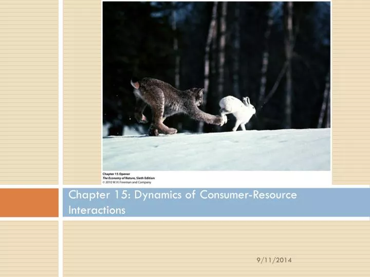
Chapter 15: Dynamics of Consumer-Resource Interactions. Population Cycles of Canadian Hare and Lynx. Charles Elton’s seminal paper focused on fluctuations of mammals in the Canadian boreal forests. Elton’s analyses were based on trapping records maintained by the Hudson’s Bay Company

E N D
Population Cycles of Canadian Hare and Lynx • Charles Elton’s seminal paper focused on fluctuations of mammals in the Canadian boreal forests. • Elton’s analyses were based on trapping records maintained by the Hudson’s Bay Company • of special interest in these records are the regular and closely linked fluctuations in populations of the lynx and its principal prey, the snowshoe hare • What causes these cycles?
Some Fundamental Questions • The basic question of population biology is: • what factors influence the size and stability of populations? • Because most species are both consumers and resources for other consumers, this basic question may be refocused: • are populations limited primarily by what they eat or by what eats them?
More Questions • Do predators reduce the size of prey populations substantially below the carrying capacity set by resources for the prey? • this question is prompted by interests in management of crop pests, game populations, and endangered species • Do the dynamics of predator-prey interactions cause populations to oscillate? • this question is prompted by observations of predator-prey cycles in nature, such as Elton’s lynx and hare
Consumers can limit resource populations. • An example: populations of cyclamen mites, a pest of strawberry crops in California, can be regulated by a predatory mite: • cyclamen mites typically invade strawberry crops soon after planting and build to damaging levels in the second year • predatory mites invade these fields in the second year and keep cyclamen mites in check • Experimental plots in which predatory mites were controlled by pesticide had cyclamen mite populations 25 times larger than untreated plots.
What makes an effective predator? • Predatory mites control populations of cyclamen mites in strawberry plantings because, like other effective predators: • they have a high reproductive capacity relative to that of their prey • they have excellent dispersal powers • they can switch to alternate food resources when their primary prey are unavailable
Consumer Control in Aquatic Ecosystems An example: sea urchins exert strong control on populations of algae in rocky shore communities: • in urchin removal experiments, the biomass of algae quickly increases: • in the absence of predation, the composition of the algal community also shifts: • large brown algae replace coralline and small green algae that can persist in the presence of predation
Predator and prey populations often cycle. • Population cycles observed in Canada are present in many species: • large herbivores (snowshoe hares, muskrat, ruffed grouse, ptarmigan) have cycles of 9-10 years: • predators of these species (red foxes, lynx, marten, mink, goshawks, owls) have similar cycles • small herbivores (voles and lemmings) have cycles of 4 years: • predators of these species (arctic foxes, rough-legged hawks, snowy owls) also have similar cycles • cycles are longer in forest, shorter in tundra
Herbivores can control plant populations • Klamath weed, or St. John’s wart, became a widespread pest following its introduction into the western US
Infestation of Klamath weed brought under control by introduced beetles
Many predator and prey populations increase and decrease in regular cycles
Why? Hare populations fluctuated less on an island with few predators than on the surrounding mainland
Other factors… • Period and intensity of a cycle also depend on the physical environment • Owl (predator) and vole (prey) population cycle dramatically over 4-year periods in northern Scandinavia – but fluctuate annually in the milder climate of southern Sweden • Why? • Prolonged heavy snow cover protects the voles from the owls thus creating a delay in the effects…
Predator-Prey Cycles: A Simple Explanation • Population cycles of predators lag slightly behind population cycles of their prey: • predators eat prey and reduce their numbers • predators go hungry and their numbers drop • with fewer predators, the remaining prey survive better and prey numbers build • with increasing numbers of prey, the predator populations also build, completing the cycle
Time Lags in Predator-Prey Systems • Delays in responses of births and deaths to an environmental change produce population cycles: • predator-prey interactions have time lags associated with the time required to produce offspring • 4-year and 9- or 10-year cycles in Canadian tundra or forests suggest that time lags should be 1 or 2 years, respectively: • these could be typical lengths of time between birth and sexual maturity • the influence of conditions in one year might not be felt until young born in that year are old enough to reproduce
Time Lags in Pathogen-Host Systems • Immune responses can create cycles of infection in certain diseases: • measles produced epidemics with a 2-year cycle in pre-vaccine human populations: • two years were required for a sufficiently large population of newly susceptible infants to accumulate
Time Lags in Pathogen-Host Systems other pathogens cycle because they kill sufficient hosts to reduce host density below the level where the pathogens can spread in the population: • such cycling is evident in polyhedrosis virus in tent caterpillars • In many regions, tent caterpillar infestations last about 2 years before the virus brings its host population under control • In other regions, infestations may last up to 9 years • Forest fragmentation – which creates abundant forest edge – tends to prolong outbreaks of the tent caterpillar • Why? • Increased forest edge exposes caterpillars to more intense sunlight inactivates the virus thus, habitat manipulation here has secondary effects
Laboratory Investigations of Predators and Prey • G.F. Gause conducted simple test-tube experiments with Paramecium (prey) and Didinium (predator): • in plain test tubes containing nutritive medium, the predator devoured all prey, then went extinct itself • in tubes with a glass wool refuge, some prey escaped predation, and the prey population reexpanded after the predator went extinct • Gause could maintain predator-prey cycles in such tubes by periodically adding more predators
Predator-prey interactions can be modeled by simple equations. • Lotka and Volterra independently developed models of predator-prey interactions in the 1920s: dR/dt = rR - cRP describes the rate of increase of the prey population, where: R is the number of prey P is the number of predators r is the prey’s per capita exponential growth rate c is a constant expressing efficiency of predation
Lotka-Volterra Predator-Prey Equations • A second equation: dP/dt = acRP - dP describes the rate of increase of the predator population, where: P is the number of predators R is the number of prey a is the efficiency of conversion of food to growth c is a constant expressing efficiency of predation d is a constant related to the death rate of predators
Predictions of Lotka-Volterra Models • Predators and prey both have equilibrium conditions (equilibrium isoclines or zero growth isoclines): • P = r/c for the predator • R = d/ac for the prey • when these values are graphed, there is a single joint equilibrium point where population sizes of predator and prey are stable: • when populations stray from joint equilibrium, they cycle with period T = 2 /rd
Cycling in Lotka-Volterra Equations • A graph with axes representing sizes of the predator and prey populations illustrates the cyclic predictions of Lotka-Volterra predator-prey equations: • a population trajectory describes the joint cyclic changes of P and R counterclockwise through the P versus R graph
Factors Changing Equilibrium Isoclines • The prey isocline increases (r/c) if: • Reproductive rate of the prey (r) increases or capture efficiency of predators (c) decreases, or both: • the prey population would be able to support the burden of a larger predator population • The predator isocline (d/ac) increases if: • Death rate (d) increases and either reproductive efficiency of predators (a) or c decreases: • more prey would be required to support the predator population
Other Lotka-Volterra Predictions • Increasing the predation efficiency (c) alone in the model reduces isoclines for predators and prey: • fewer prey would be needed to sustain a given capture rate • the prey population would be less able to support the more efficient predator • Increasing the birth rate of the prey (r) should lead to an increase in the population of predators but not the prey themselves.
An increase in the birth rate of prey increases the predator population but not the prey population.
Modification of Lotka-Volterra Models for Predators and Prey • There are various concerns with the Lotka-Volterra equations: • the lack of any forces tending to restore the populations to the joint equilibrium: • this condition is referred to as a neutral equilibrium • the lack of any satiation of predators: • each predator consumes a constant proportion of the prey population regardless of its density
The Functional Response • A more realistic description of predator behavior incorporates alternative functional responses, proposed by C.S. Holling: • type I response: rate of consumption per predator is proportional to prey density (no satiation) • type II response: number of prey consumed per predator increases rapidly, then plateaus with increasing prey density • type III response: like type II, except predator response to prey is depressed at low prey density
Welcome back • Yes, exam is on the 23rd of December • Chapters 7, 8, 10, 14, 15 + cc • http://www.guardian.co.uk/environment/interactive/2009/dec/07/copenhagen-climate-change-carbon-emissions • Exam is in this class room. Promptly at 2 pm • Oral presentations • I may miss you Friday (not 100% sure) • Remaining chapters • Chapters 22, 23, 26, 27 plus ?
Student Exam questions • submit ?s to me via email that could be used on the exam. Submit ?s by 21-December (Mon) • The ?s should have the same format as those on the practice quizzes (i.e., multiple choice with 4 options). You may also email essay questions. • Put "BIOL 207: questions for exam" in the subject line. For each ? of yours that is used on the exam, you will receive 1 EC pt. I will limit you to 2 EC ? per exam, but it is in your best interest to submit several (8-10) ?s.
Lotka-Volterra model (remember?) • [the rate of change in the prey population ] = [the intrinsic growth rate of the prey population] – [the removal of prey individuals by predators] • Equilibrium isocline