Download
1 / 28
280 likes | 401 Views
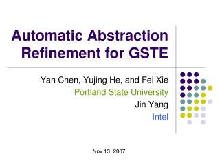
A Logic for GSTE. Edward Smith University of Oxford. X. 0. s. 0. s. 1. Generalized Symbolic Trajectory Evaluation (GSTE). Based on gate-level simulation Ternary simulation over {0,1,X} Symbolic simulation layer Fine control over abstraction Fixed-points allow unbounded properties

E N D
A Logic for GSTE Edward Smith University of Oxford
X 0 s 0 s 1 Generalized Symbolic Trajectory Evaluation (GSTE) • Based on gate-level simulation • Ternary simulation over {0,1,X} • Symbolic simulation layer • Fine control over abstraction • Fixed-points allow unbounded properties • Regular properties
Traditional Specification • Using assertion graphs • Shape and labels drive model checking • Affect efficiency and abstraction level Drive input A Assert correct output Drive input B
Verification Process High-level Specification An example specification For a simple GSTEproperty that isn’t too hard to verify I hope, but you never really know, Hopefully not Assertion Graph Manually Refine or Decompose GSTE Fails GSTE Succeeds Circuit
Verification Process Rules difficult to express, apply and justify High-level Specification An example specification For a simple GSTEproperty that isn’t too hard to verify I hope, but you never really know, Hopefully not Assertion Graph Manually Refine or Decompose GSTE Fails GSTE Succeeds Circuit
k b c k f f f Generalized Trajectory Logic • A clean specification notation based on temporal logic • Trace-based semantics • Symbolic set of words • What we check • GSTE simulation state • Upper-approximation • How we simulate
+ ( ( ) ) K N K S T S µ t 2 n r a c e s = ; Circuit Model • Kripke structure • Nodes
+ + + f ; b f k c k j j ( ( ) g ) g X ? X f f X f f X f X X X X X X S S S 0 1 t t 2 2 n n n n : ¾ ¾ s s : s s : : : : : : : : : : : Formulas of GTL
k b k b k b c c c k k k b b k k c c k k f X f f X X h h X X h h X h h X X X X 0 1 1 0 0 0 0 1 ^ _ t u t u \ [ g g g g g g = = Formulas of GTL
+ f k b c k ( b c ) j k k g f f f Y Y S t 2 2 g s ¾ e g g p s g ¾ g : Yesterday • Allows compositional simulation forward step simulate g
( b b ( j ) j j c ) ( ) c f f f h h h h l h l X X X X I Q Q Q Q 1 1 t n n n n e e g g u w : e u r u e g e n u g e a s s : e v : a u e u : u ! = ! ! = = = . . . . : : : : : : Symbolic Formulas
( ) ( ( ) ) ( ) f f h f f b d f f Y Z Z Z i i w e r e g n g s g e v e r y n ¹ g g ; ; : : : : Fixed-points • Mu-calculus style fixed-points capture iteration
( ) ( ( ( ) ) ) ( ) f f f h f f f b d f f f f P S Y Y Y Z Z Z Z Z Z Z i i _ _ ^ w e g r e : g : ¹ ¹ n g s g g e v e r y n ¹ g g = = ; ; : : : : : : Fixed-points • Mu-calculus style fixed-points capture iteration • E.g. ‘Previously f’ and ‘f Since g’
( ) Y Z E R O O N E t t _ ^ r e s e r e s e : = ( ) Y O N E Z E R O t ^ r e s e : = Vector Fixed-points • Nested mu-expressions are messy in practice • Fixed-points are unique • Can therefore use systems of recursive equations:
( ( ) ) ( ( ( ) ) ( j ( ) ) ) 9 f i f f Q Q T F _ n s n n u : : u : : u : = = = ! = : ( ) ( ( ) ) ( ( ) ) 8 f f f T F ^ u : u : u : = = = : Shorthand • Quantification • Calculated directly using BDD quantification • Symbolic node value
k ( ( k ) ( ( k k ) ) ) d l i d i d S A C A C i i i t t t ^ ^ 2 2 r e a w r w r n s o u s : m p e s ) ) GTL Properties when, for every trace t and in every symbolic valuation: e.g. Register correctness:
b c b c l A C A C i i v m p e s ) Model Checking Upper-approximation simulation Precise simulation, when C does not contain disjunction or Y
b c ( ) b c ( ( ( ) ) ) f f f f f f 6 f f f f f f f f Y Y Y Z Z Z Z ^ ^ ^ ^ ^ ^ n n ¹ g : g g g g ¹ g = = = = = = : : Reasoning with GTL • Simple rules for traced-based equivalence • Rules do not imply simulation equivalence • Property-preserving simulation transformations
( ) [ / ] f f f f f f Q Q ^ g u : u = = = Optimization Rules • Simplification, e.g. • Symbolic/explicit conversion
( ( ( j j ) ( ) ) ) ( ( j ) ( ) ) 9 1 0 _ _ n n n n n n n n n n n s s : s : : s : s : s : ! ! = ! = : Example 0 1 f s 1 f 1 1 f = =
A A B C B A C C A C A A B C C ) ) ) ) 1 1 2 2 2 1 2 1 A C [ = ] A A C C ) ) 2 1 1 2 Decomposition Rules • Transitivity connects simulations • Monotonicity connects branching simulations
( ( ) ) ( ) ( ) - - - f f f f h f f h Y Y Y Y _ ^ _ ^ _ g g g g g Abstraction Refinement • ‘Less abstract than’ relation • Only and lose information Information loss occurs earlier in simulation
a a a a a a a a a b b b b b b b b b ( ) b b b b b b Y Y Y Y Y ^ ^ ^ a a a a a a 1 1 1 1 1 1 1 1 • Affects which circuit segments are simulated independently
Conclusions • GTL is a temporal logic for GSTE • Textual form is easier to manage • Fine granularity induces algebraic nature • Logical rules express sound refinements • Simple rules exist for decomposition/refinement
( ) f f f f P S Y Y Z Z Z Z _ _ ^ g : : ¹ ¹ g = = : : • Previously f • f Since g
( ) Y Z E R O O N E t _ r e s e : = ( ) Y O N E Z E R O = • Fixed-points are unique • Can also use systems of equations, e.g.
I I µ [ [ \ \ m m Our Approach Assertion Graph: Simulation Steps: • Describe these atomic steps in a logical form • Hope to gain reasoning rules