Download
1 / 32
320 likes | 392 Views
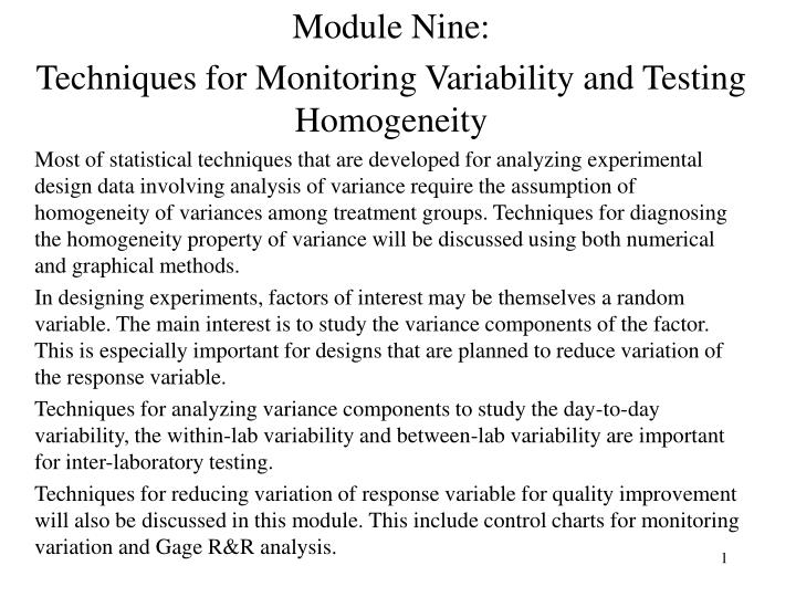
Module Nine: Techniques for Monitoring Variability and Testing Homogeneity

E N D
Module Nine: Techniques for Monitoring Variability and Testing Homogeneity Most of statistical techniques that are developed for analyzing experimental design data involving analysis of variance require the assumption of homogeneity of variances among treatment groups. Techniques for diagnosing the homogeneity property of variance will be discussed using both numerical and graphical methods. In designing experiments, factors of interest may be themselves a random variable. The main interest is to study the variance components of the factor. This is especially important for designs that are planned to reduce variation of the response variable. Techniques for analyzing variance components to study the day-to-day variability, the within-lab variability and between-lab variability are important for inter-laboratory testing. Techniques for reducing variation of response variable for quality improvement will also be discussed in this module. This include control charts for monitoring variation and Gage R&R analysis.
Presenting uncertainty for sample variance: 100(1-a)% Confidence Interval for Population Variance, s2 • In an inter-laboratory testing study, we often encounter the problem of estimating within-lab variability and between-lab variability. These are used to study the ‘repeatability’ and ‘reproducibility’ of a testing procedure. • Repeatability refers to how well a test procedure can be repeated for testing the same material under the same condition in the same laboratory. It is often measured by the within-lab variability when the testing environment and experimental units are as homogeneous as possible. Hence, it measures the uncertainty due to the combined small uncontrollable random errors. • Reproducibility refers to how well a measurement of the same material using the same testing procedure can be reproduced in different laboratories. • When a lab is under a good statistical control, the sources of special causes are minimum, therefore, the repeatability is expected to be high. • Reproducibility is more complicated. The low reproducibility often reflected by the large between-lab variability. The causes of low reproducibility may be due to material itself, the difference between labs in the environmental conditions, operator’s training, and systematic errors. • How to measure the repeatability and reproducibility is important in a inter-laboratory study or in a gauge analysis.
To discuss the presentation of variation, we start from one sample case. Consider we observe n testing results of a material using a testing procedure by repeatedly testing the material for n times. One task is to measure the repeatability of the testing procedure for the same material. A simple and useful estimate of the repeatability is the variance, s2, and the standard deviation, s. Different from measuring the uncertainty of sample mean, since sample variance, s2 is always non-negative, we do not report the uncertainty of s2 in the form of In stead, based on some statistical theory, when the sample is drawn from a normal population, the distribution of s2 can be determined by a so-called Chi-Square distribution:
Statistically, (Chi-square)distribution with degrees of freedom is a continuous probability distribution with probability density: f(x) x 5 10 15 What is Chi-Square Random Variable? What does the distribution look like? How to compute Ch-square Probability or use Chi-square Table?
Hands-on Activity of using Chi-square Table and using Minitab to find the Chi-square quantiles. • df = 20, find 95th percentile , P( < Q(.95) = .95 • More examples here, if needed.
The uncertainty of using s2 to estimate s2can be expressed in terms of 100(1-a)% confidence interval. After some simple algebra, we obtain a 100(1-a)% confidence interval for s2: Lower Bound = Upper Bound = Where, Case Example: The TAPPI Data : Sample GR36. 76 labs tested the sample GR36. The sample variance and standard deviation are s2 = .4679, s = .684 A 95% confidence interval for the lab variation is Lower bound = (76-1)(.4679)/100.84 = .348 Upper bound = (76-1)(.4679)/50.94 = .689 95% sure that the lab variance is between .348 to .689
Hands-on activity • It was found that three labs may have large within –lab variability. An experiment was conduct at these three labs to test the same material. Each material was tested for 20 times. The sample s.d. is found to be: • sA = 4.5 sB = 8.4 sc=5.6 • (a) Obtain a 95% confidence interval to estimate the within-lab variance, respectively. • (b) Is there overlap between the 95% confidence interval for Lab A and Lab B? • (c ) Based on the result in (b), is there a strong evidence to conclude that the within-lab variance of Lab B is significantly higher than that of Lab A?
Comparing the homogeneity of variances between two groups • When two materials are tested for n repetitions in the same lab, we are often interested in investigating two aspects about the testing results: • To compare the average testing results between two materials (this was done in Module Eight). The approach is the t-test. • To compare the within-material variability of the testing results. • The second type of comparison is to compare the ratio of variances between two groups, : Our goal is to estimate this ratio based on two independent samples, one from each population. Notice that, in order to measure the uncertainty of the ratio, , we compute the ratio of sample variances: . Similar to the measurement of one-sample variance, we need to understand the corresponding distribution of or some function of that will allow us to study the uncertainty of measuring
The idea is to take two independent samples and compute sample variances to make inference about Assuming that each sample data are observed independently from a normal population, statistical theory tells us the ratio of sample variance, follows so-called F-distribution with numerator degrees of freedom (df) being the df of and denominator df being the df of That is, F= , and the F-distribution depends on df1 = numerator df, and df2 = denominator df. For this two material testing example, df1 = (n-1) = df2
f(x) x What is F-distribution? What does it look like? How to compute the cumulative probability or quantiles using Table and using Minitab Statistically, F-distribution with numerator and denominator degrees of freedom is a continuous probability distribution with probability density:
Hands-on Activity : Using F-Table • An important property of F-distribution: Because of this property, most of F-quantile tables only present either the upper or lower end of the F-distribution. This property is used to determine the other end of the F-quantiles. Exercises of using F-table may be needed here.
Using the F-distribution, we are able to test the hypothesis at the level of significance, a: • Compute • Obtain the critical F-value using F-Table or software such as Minitab. The critical values for two-side test are • F(a/2, df1,df2), and F(1-a/2,df1,df2) • When Fobs falls outside the two critical values, we conclude that the two population variances are significantly different. • (Note: Hypothesis test can also be a right-side test or a left-side test.) • If we use software for conduct this comparison, software such as Minitab gives us what so-called p-value. It is the observed level of significance. Therefore, to make a decision, we can compare p-value with a using the rule: • If p-value < a, then, reject Ho, , two variances are significantly different. • If p-value a , then, do not reject Ho, the variances are not significantly different.
100(1-a)% confidence of the ratio can also be established to estimate the uncertainty of the ratio: F-distribution describes the distribution of Where, two independent samples of size n1 and n2 are randomly chosen from a normal populations with variances Rearranging in the following probability inequality one obtains 100(1-a)% confidence interval for : Lower Bound = Upper Bound =
Hands-On Activity A study was conducted to compare the water-insoluble nitrogen in two type of fertilizers. Type A was randomly assigned to ten labs, and Type B was randomly assigned to test Type B. Assuming labs have little systematic error. The tested results are summarized: • Obtain a 90% confidence interval for ratio of variances of the two types of fertilizers. • Test if type A has a significantly lower variance when compare with Type B using a = 1%.
A more robust method for testing the uniformity of variances Levene’s Test This method considers the distances of the observations from their sample median rather than their sample mean. Using the sample median rather than the sample mean makes the test more robust for smaller samples as well as making the procedure asymptotically distribution-free. The test statistic is given by: ni is the number of observations for the ith sample. N is the total numbers of observations, Levene’s test statistic FL follows an F-distribution with numerator d.f., n1 = k-1 and denominator d.f., n2 = N-k For two population case, k = 2. The decision rule is: When the observed FL > F(a, 1, N-2), Two variances are concluded not uniform.
The measurement uncertainty of variance is different from the measurement uncertainty of mean. In addition, because of the distribution properties, the interval of the measurement uncertainty is presented in terms of confidence interval, in stead of only based on The confidence intervals are developed rather differently between mean and variance. The sample mean is based on While confidence interval for variance is based on ratio uncertainty. The general approach of measuring uncertainty for f(x1,x2, …., xk) require little assumption, therefore, the measurement uncertainty based on the general approach is usually more conservative. As a consequence, the measurement uncertainty is usually larger. One should take the advantage of the distribution property, if the distribution of the variable can be approximated properly, such as Normal, t, Ch-square, and F-distributions, and so on. The measured uncertainty will be more precise. However, if the assumption, which we have been making, ‘the population from which we draw the sample follows a normal curve’ or ‘ the sample size is large’ is not satisfied, the results may be too optimistic or even inappropriate. Therefore, a quick diagnosis of distribution and outliers are important. Or use tests that are more robust to the violation of normal assumption can be used. For the Two population variances problem, Levene’s FL-test can be applied.
Use Minitab to construct confidence interval estimate for variance: • Consider the following example: The uniformity of hardness of specimen of 4% carbon steel is a key quality characteristics. Two types of steels are to be compared: Heat-Treated and Cold-Rolled. There are typically two important questions to be answered: • Which type of steel has higher hardness? – A problem of comparing the means using t-test. • Which one gives more uniform hardness? - A problem of comparing the variances using the F-test or Levene’s Test. • In the following, we will use Minitab to conduct the analysis for problem (2) and leave problem (1) as a hands-on activity. • In Minitab: • Go to Stat, choose Basic Statistics, then select ‘2 variances’. • Depending on how the data are organized. If the data are in two columns, click on ‘Samples in different columns’, and enter the variables. • Click on ‘Options’, it allows you to enter the level of confidence. By default, it is 95%. • Storage selection allows you to store some computed results.
Row Heat-Tr Cold-Tr 1 31.8 21.1 2 43.7 24.9 3 35.6 19.8 4 38.0 16.5 5 24.5 18.3 6 29.5 20.9 7 38.9 16.4 8 32.4 17.3 9 29.5 15.8 10 19.7 17.6 11 24.6 14.6 12 39.7 23.4 13 42.5 19.4 14 40.6 20.6 15 32.6 17.8 16 36.8 17 37.5 18 33.1 19 31.8 20 28.7 Variable N Mean Median StDev SE Mean Min Max Heat-Tr 20 33.58 32.85 6.36 1.42 19.7 43.7 Cold-Tr 15 18.96 18.30 2.87 0.74 14.6 24.9
Test for Equal Variances Level1 Heat-Tr Level2 Cold-Tr ConfLvl 95.0000 Bonferroni confidence intervals for standard deviations Lower Sigma Upper N Factor Levels 4.65829 6.35832 9.85093 20 Heat-Tr 2.01077 2.86501 4.85604 15 Cold-Tr F-Test (normal distribution) Test Statistic: 4.925 P-Value : 0.004 Levene's Test (any continuous distribution) Test Statistic: 7.123 P-Value : 0.012 \Workshop-Taiwan-Summer-2001\Data Sets\Steel-treat-conf-var.MPJ Both F-test and Levene’s test show the two types of steel have significantly different uniformity. In particular, the Heat-Treated is much higher than the Cold-Rolled steel. 95% Bonferroni confidence intervals are also provided. It shown that 95% of chance that the hardness non-uniformity of Heated-steel measured by s.d. is from 4.65 to 9.85. While the non-uniformity of Cold-Rolled steel is from 2.01 to 4.86.
What is the Bonferroni’s Simultaneous Confidence Interval? How to construct them? How to interpret them? • Bonferroni’s simultaneous confidence interval for s.d. as reported in the Minitab modifies the confidence interval for each individual sample variance using Chi-square distribution. The method is described in the following: • For each group, compute sample variances, si2, I = 1,2, …, k. • When constructing an individual using Chi-square, the critical values are modified depending on the number of confidence intervals to be constructed: Lower Bound = Upper Bound =
NOTE: For single confidence interval, k=1, the confidence interval is the same as we discussed before. When we have more than one intervals, in order to keep the type I error to be still a, Bonferroni proposed to reduce the type I error for a member of the confidence intervals to be a/2k. Example- Using the Steel data, we obtain: 95% Bonferroni confidence intervals for standard deviations Lower Sigma Upper N Factor Levels 4.65829 6.35832 9.85093 20 Heat-Tr 2.01077 2.86501 4.85604 15 Cold-Tr The Lower Bound 4.6583 for s1 is obtained by The corresponding Chi-square values are: 35.3986 and 7.9156, and the upper bound is found to be 9.8509
Hands-on Activity Construct the Bnoferroni confidence interval for the Cold-Rolled type of steel.
The graphical presentation of the comparison are also provided by Minitab in the following.
The uniformity of hardness of steel is a classical example in quality improvement • To improve the hardness – the harder the better. • That is to improve the signal of the quality characteristic. • To reduce the non-uniformity – minimize the variability – the smaller the s.d., the better. • That is to reduce the noise of the quality characteristic. • This is one of the major contributions due to Taguchi, who proposed what is now known as Signal-to-Noise Ratio analysis in quality improvement.
Hands-on Activity • Use the Hardness of Steel data to conduct the following analysis: • Test if the hardness of two types of steel is significantly different. • Suppose the standard hardness of steel for bridge is at the minimum of 25. Does either of the steel meet the standard? • Suppose the standard variability of the hardness of steel is at the maximum of 4.5. Does either type of steel meet this requirement?
Testing homogeneity of variability for more than two groups (Testing for uniformity of measurements for more than two groups) • In real world applications, including the laboratory testing, it often the case that there are more than two groups for comparison. As a result, we need methods for making comparison among three or more groups. • Testing for homogeneity of variances is important for at least two purposes: • The homogeneity of variances reflects to the quality of the variable of interest. This is especially important in quality improvement. For the example of uniformity of hardness of steel. If the steel has a huge variation of the hardness, the life time of buildings or bridges will be very unreliable. Some lots of steel may last for 50 years, while others may only last for 10 years due to the hardness variation of the same type of steel. • In making an appropriate comparison of group means, we often make the assumption that the within-group variation is constant. That is, the within-group variations are approximately similar. Therefore, an appropriate comparison of group means requires a diagnosis of homogeneity of variance.
ni is the number of observations for the ith sample. N is the total numbers of observations, Levene’s test statistic FL follows an F-distribution with numerator d.f., n1 = k-1 and denominator d.f., n2 = N-k The decision rule is: When the observed FL > F(a, k-1, N-k), the within-group variances are concluded not uniform. Levene’s Test and Bartlett’s Test for testing homogeneity of variances of more than two groups We have introduced Levene’s FL-test for two group comparison. This test is good for more than two groups as the formula shows.
Bartlett’s Test for Homogeneity of Variances Consider we have three types of steel, and we are interested in comparing the uniformity of the hardness. To do so, we conduct a lab experiment to test the hardness of three types of steel. The data is recorded in table form such as: Bartlett Test is based on the nature log transformation of the geometric mean of the sample variances. If within-group variances are all equal, we can estimate the overall variance by combining all of the k groups of data together. As a consequence, the difference between the combined variance and the uncombined variance gives the basis for the bartlett test.
Row Cold-Tr Mid-Tr Heat-Tr 1 21.1 30.4 31.8 2 24.9 27.5 43.7 3 19.8 21.8 35.6 4 16.5 24.9 38.0 5 18.3 31.4 24.5 6 20.9 18.5 29.5 7 16.4 16.7 38.9 8 17.3 19.8 32.4 9 15.8 23.8 29.5 10 17.6 25.7 19.7 11 14.6 29.4 24.6 12 23.4 28.4 39.7 13 19.4 21.7 42.5 14 20.6 26.4 40.6 15 17.8 30.6 32.6 16 36.8 17 37.5 18 33.1 19 31.8 20 28.7 \Workshop-Taiwan-Summer-2001\Data Sets\Steel-treat-conf-var.MP Variable N Mean Median StDev SE Mean Min Max Heat-Tr 20 33.58 32.85 6.36 1.42 19.7 43.7 Cold-Tr 15 18.96 18.30 2.87 0.74 14.6 24.9 Mid-Tr 15 25.13 25.70 4.64 1.20 16.7 31.4
Test for Equal Variances: Response Hardness ConfLvl 95.0000 Bonferroni confidence intervals for standard deviations Lower Sigma Upper N Factor Levels 1.96631 2.86501 5.0557 15 Cold-Tr 4.56689 6.35832 10.1796 20 Heat-Tr 3.18546 4.64138 8.1903 15 Mid-Tr Bartlett's Test (normal distribution) Test Statistic: 8.676 P-Value : 0.013 Levene's Test (any continuous distribution) Test Statistic: 3.927 P-Value : 0.026 Both Bartlett test and Levene test conclude that the with-group variances are not uniform. Note that Bartlett test requires Normality assumption of the population. Levene Test does not require this assumption.
A graphical presentation of testing homogeneity of variances
Hands-on Activity • Perform the following test by hand using the steel data: • Bonferroni’s simultaneous confidence interval for the Mid-temperature treated steel. • Perform the Bartlett test. • Perform the Levene test.