Download
1 / 14
140 likes | 188 Views
Stress and social class. | class stress | Low Middle Upper | Total -----------+---------------------------------+---------- Low | 246 90 55 | 391 | 62.92 23.02 14.07 | 100.00

E N D
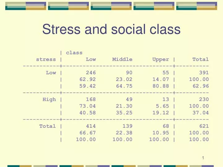
Stress and social class | class stress | Low Middle Upper | Total -----------+---------------------------------+---------- Low | 246 90 55 | 391 | 62.92 23.02 14.07 | 100.00 | 59.42 64.75 80.88 | 62.96 -----------+---------------------------------+---------- High | 168 49 13 | 230 | 73.04 21.30 5.65 | 100.00 | 40.58 35.25 19.12 | 37.04 -----------+---------------------------------+---------- Total | 414 139 68 | 621 | 66.67 22.38 10.95 | 100.00 | 100.00 100.00 100.00 | 100.00
Independence • Two variables, A and B, are independent if p(A) = p(A|B) • p(Stress) = .37, p(Stress|Hi class) = .19 • Also, note • p(s|low) = .41 p(s|mid) = .35 p(s|hi) = .19 • Also note, these are from the appropriate percentages, since class causes stress.
Independence • If there is independence, then • p(s) = p(s|lo) = p(s|mid) = p(s|hi) • What would the frequencies be if there was independence? • p(s) = .37 = p(s|lo) = p(s|mid) = p(s|hi) • This .37 is taken from the margin (unconditional probability of stress)
Apply this | class stress | Low Middle Upper | Total -----------+---------------------------------+---------- Low | 246 90 55 | 391 | 62.96 62.96 62.96 | 62.96 | 260.65 87.52 42.81 | -----------+---------------------------------+---------- High | 168 49 13 | 230 | 37.04 37.04 37.04 | 37.04 | 153.35 51.48 25.19 | -----------+---------------------------------+---------- Total | 414 139 68 | 621 | 100.00 100.00 100.00 | 100.00
Observed and Expected • Are they the same? • Then p(s) = p(s|class) -- Independence • Are they different? • Then p(s) ‡ p(s|class) -- Relationship • How can we tell?
Look at parts of formula What if we just sum difference without squaring? How big is a difference of 5 points? What happens when there are lots of cells in the table we are looking at?
Look again • This sum has a chi-square distribution • Like the t-distribution, chi-square has a different shape for each different degrees of freedom • More cells, bigger sum
Degrees of freedom • For independence tests between two categorical variables • df = (rows-1) time (cols-1) • For other tests using the chi-square distribution df is calculated differently. We will cover them.
Looking at our data | class stress | Low Middle Upper | Total -----------+---------------------------------+---------- Low | 246 90 55 | 391 | 62.96 62.96 62.96 | 62.96 | 260.65 87.52 42.81 | -----------+---------------------------------+---------- High | 168 49 13 | 230 | 37.04 37.04 37.04 | 37.04 | 153.35 51.48 25.19 | -----------+---------------------------------+---------- Total | 414 139 68 | 621 | 100.00 100.00 100.00 | 100.00 Observed Expected Observed Expected
Calculations Obs Exp Diff Diff Sq Diff Sq / Exp 246 260.65 -14.65 214.62 0.82 90 87.52 2.48 6.15 0.07 55 42.81 12.19 148.60 3.47 168 153.35 14.65 214.62 1.39 49 51.58 -2.48 6.15 0.12 13 25.19 -12.19 148.60 5.90 Sum (Chi-Square) = 11.77 df (3-1)(2-1) = 2 critical chi-square at 95% (from table) 5.99
Decision Chi-square distribution with 2 df Critical Region Sample chi-square 5.99
A single variable • Tossing a coin 100 times, we observe 57 heads. Could this occur by chance? • Observed 43 and 57 • Expected 50 and 50 -- why is this so? • Chi-square (43-50) / 50 + (57-50) / 50 = 2.0 • df = (rows-1) -- there are no columns • Critical (95%) chi-square with df=1 is 3.84 • Decision: could happen by chance
Comparing two proportions • Do tenured faculty get a larger proportion of small classes than untenured faculty? • Null hypothesis is proportions are the same • This makes a fourfold table (2x2) • Null hypothesis is equivalent to independence between tenure status and class size
Table from text Faculty Class Size Status Small Large Total Untenured 9 (.64) 7 (.44) 16 (.53) Tenured 5 (.36) 9 (.56) 14 (.47) Total 14 18 30 Chi-square = 1.265 df (rows-1)(cols-1) = 1 Critical (95%) value of chi-square 3.84 Decision: fail to reject null hypothesis of independence