Pietro Armienti and Daniela Gasperini (Università di Pisa) based on the papers

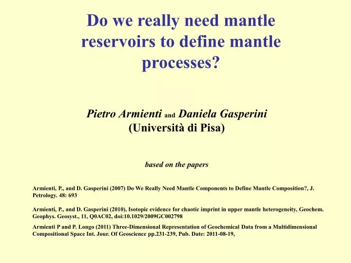
1. Do we really need mantle reservoirs to define mantle processes? Pietro ArmientiandDaniela Gasperini(Università di Pisa)based on the papers Armienti, P., and D. Gasperini (2007) Do We Really Need Mantle Components to Define Mantle Composition?, J. Petrology. 48: 693 Armienti, P., and D. Gasperini (2010), Isotopic evidence for chaotic imprint in upper mantle heterogeneity, Geochem. Geophys. Geosyst., 11, Q0AC02, doi:10.1029/2009GC002798 Armienti P and P. Longo (2011) Three-Dimensional Representation of Geochemical Data from a Multidimensional Compositional Space Int. Jour. Of Geoscience pp.231-239, Pub. Date: 2011-08-19,

2. This analysis is based on an algorithm which projects data from multi-dimensional space to three-dimensions

3. The projection scheme from Rn to R3 may be illustrated by the analogy of projecting from a plane onto a segment AB. y In 2D space two points B, A define the 1D space onto which E (x,y) is mapped onto E* (e). E l v 1 1 E* A B v = A - B 1 l A E* = B + v B 1 1 x

4. Similarly, four points define the 3D space onto which data can be projected from Rn For simplicity, the four points (“end-members”) are mapped onto the vertices of a regular tetrahedron

5. A suitable set of four end-members, each defined by its components (e.g. minerals & major elements), defines a suitable tetrahedron. Points with negative values, required to obey mass-balance constraints, may also be projected.

6. This also allows data to be projected onto the face of the tetrahedron opposite a particular vertex.The same scheme allows also relevant phase relations to be projected in petrologic diagrams

7. Click to get :The paper the source program and instructions

8. OIB data • We selected about 1700 analyses of tholeiites, picrites, foidites, basanites and alkaline basalts from different oceanic islands from the GEOROC database (http://georoc.mpch-mainz.gwdg.de/Start.asp). Loss on ignition is less than 2.2 wt% and Mg# > 63 for all analyses. • All the samples were re-classified according to IUGS recommendations (Le Maitre, 1989) due to discrepancies in the classifications reported by the AA. • After reclassifying the analyses in terms of their CMAS components, the data were projected from Di, using the method described above.

9. Alkali Basalt Nephelinite Basanite Basaltic Tholeiite Picrobasalt Garnets Projection of major element data onto the CaTs-Ol-Q face of the CaTs-Ol-Di tetrahedron was done by reclassifying the major element data according to O’Hara (1968) and the molecular proportions of the table in Slide 7. The CaTs-En line acts as a thermal divide at pressures exceeding 2 GPa and separates critically undersaturated compositions from Hy-normative ones. The Ol-An join separates Hy-normative lavas from Ol-Hy-normative ones. The grey line separates partial melts attributed to a peridotitic source (those below the gray line) from those derived from partial melting of a pyroxenitic source.

10. Nephelinite Basanite Alkali Basalt Tholeiite CaTs An CaTs 1.5 2-2.5 1 2 2.5 3-3.5 Q Ol (a) overview of experimental data on partial melts. Numbers are pressures in GPa: 1) pyroxenites (Hirschmann et al., 2003), 2) Garnet-pyroxenites (Falloon et al., 2001), 3) pyroxenite (Keshav et al., 2004), 4-5) pyroxenite (Hirose & Kushiro, 1993; Falloon et al., 1997). (b) Fields of primitive (Mg# > 63) magmas from OIB settings; data from the GEOROC database (http://georoc.mpch-mainz.gwdg.de/Start.asp). (c) CaTs-En is a thermal divide above 2 GPa.

11. Relevant Issues • The continuous distribution of near primary melts in the Ol-CaTs-Qz diagram suggests a similar continuous variation in mineralogy of the OIB source-mantle, since melt compositions are not influenced by the divide between partial melts attributed to pyroxenitic and peridotitic sources; • The low-melting-point portions of a heterogeneous mantle may be silica-poor Gt-pyroxenite, whose partial melts are Ne-normative up to moderate degrees of partial melting (F = 0.18-0.21), then continuously evolve towards silica-rich compositions for F ≥ 0.7. Thus, the transition from alkali basalt to tholeiite may be continuous and, within a relatively small mantle volume, it may be possible to generate both mildly alkaline basalts and tholeiitic melts; • Interaction of melts derived from pyroxenite with partial melts from a peridotitic mantle may be the rule rather than the exception, and partial melting starting in low-melting-point domains may progressively extend to wider and wider mantle portions.

12. Relevant Issues Each basaltic magma generated under such conditions carries an isotope signature inherited from the mantle portions in which partial melting occurred. Under these conditions, specific compositions related to distinct mantle reservoirs are difficult to identify!

13. Three-dimensional plot of Sr, Nd and Pb (206Pb/204Pb) for worldwide OIB and MORB (http://georoc.mpch-mainz.gwdg.de/Start.asp), [Hart et al. (1992) classification] for the four end-members/vertices DMM, EMI, EMII, HIMU (table below). From a mathematical point of view, OIB data within the tetrahedron, being a convex sum of the four end-members, could represent a physical mixture of the adopted end-members.

14. For the same data, the addition of 1 compositional parameter (here 207Pb/204Pb) to the 4 components causes loss of data convexity (i.e. points cannot be a physical mixture of the end members shown in the table). Points describe sub-parallel alignments between distinctive "enriched" and "depleted" compositions, independent of the 4 end-members of Hart et al. (1992). The OIB trends mostly lie on a plane, suggesting that OIB compositional variability results basically from two degrees of freedom. ratio MORB (DMM) EMI EM2 HIMU 87 8 6 Sr/ Sr * 0.70200 0.70530 0.70780 0.70285 143 144 Nd/ Nd * 0.51330 0.51236 0.51258 0.51285 206 204 Pb/ Pb * 18.00 17.40 19.00 21.80 207 204 Pb/ Pb * 15.39 15.47 15.61 15.86

15. Some OIBs, along with pelagic sediments, spread with respect to the pseudo-plane. End-members A-D and components (n=6) are given in the table below A A D B C In the inset, the distribution on the pseudo-plane of Hawaii samples shows that picrites, along with OIB tholeiites and some alkali basalts, cluster close to the “depleted” component. Conversely, nephelinites, basanites and most alkali basalts spread on OIB arrays that drift from the picrite/tholeiite trend, towards the “enriched” composition C B D nephelinites

16. A different tetrahedron orientation for the same data set, shows the distribution of samples on the pseudo-plane wrt their origin. Magmatic suites describe sub-parallel alignments, fitting mixing curves between diverse pairs of “enriched-depleted” compositions that are distinctive for each archipelago. The equation of the mixing line drawn is z = 0.0535y2 + 0.5121y - 128.55.

17. Compositions of the 4 end-members are the same as before but 206Pb/204Pb has been dropped. The pseudo-plane collapses to an alignment if Pb isotope ratios are excluded. This suggests that OIB compositional variability is related to time- dependent Pb isotope systematics. Data dispersion along the mixing line in R3, can be clearly seen by rotation around the z and y axes.

18. Conclusions • Data projection allows a comprehensive overview of geochemical heterogeneity of OIB mantle sources. Simultaneous consideration of many compositional parameters discloses a simple scenario in which mantle heterogeneity results from a range of processes which cause incompatible element enrichment and depletion, where time plays a major role. • Different degrees of partial melting of peridotite, pyroxenite and recycled eclogite contribute to OIB petrogenesis. The geochemical signature of the enriched component, often deriving from recycled lithosphere with a distinctive age and Pb isotope signature, is crucial to characterize specific OIB mantle sources. • Extreme depleted and enriched compositions in the mantle coexist, unique to each ocean island. These are not related to the so-called mantle components DMM, EMI, EMII and HIMU. Multi-dimensional evaluation of OIB mantle sources enables us to move from a perspective based on physically distinct mantle reservoirs to one based on a marble-cake mantle structure. • Although this model is consistent with the SUMA (Statistical Upper Mantle Assemblage) model of Meibom & Anderson (2003), the highest degrees of partial melting of the mantle source of each ocean island can only reveal the distinctive local depleted source composition, precluding the existence of a mantle-wide, common depleted reservoir DMM. • This evaluation reveals that the so-called mantle components (DMM, EMI, EMII, HIMU) are significant only in the Sr, Nd, Pb perspective.

19. So, do we really need mantle reservoirs to define mantle processes?Maybe Not…!

20. What else about mantle heterogeneity? We tested the variability of the MORB mantle source as sampled by basalts collected at the EPR and MAR. Sample locations are shown as triangles. Isotope data are from PetDB and GeoROC, and from Agranier et al. (2005). Isotope data structure was explored as a space series.

21. The fractal nature of a time or space series may be revealed by suitable mathematical techniques. A 1D time or space series can be expanded into higher-dimensional space, in which the dynamic of the underlying generator may be revealed.

22. Recursive plots To expand a 1D signal into an m-dimensional phase space, each observation in the original signal X(i) has to be substituted with the vector: X(i) = x(i), x(i + l), x(i + 2l), … , x[i + (m-1)l], where i is the space (time) index, m is the embedding dimension and l is a given delay. A practical example is given in the following slide, where 2D phase space is generated by means of a recursive plot.

23. How to make a recursive plot With reference to the table at left: • Step 1 considers the values in columns A and B. A may represent a distance, B a compositional variable. • Step 2 orders B values wrt to A • Step 3 shifts column Bl steps (l is the delay of the previous slide, here l=3) • Step 4 aligns columns B and C; a plot of B vs C is a 2D (embedding dimension m=2) phase space of the series B. • If the state of the system at a given step depends on its previous conditions some relations must exist between C and B. In this case the system has an attractor, as shown in the next slide.

24. C C b a B B The fingerprints of CHAOS Recurrence plots for (a) white noise = no dependence on preceding states, and (b) the Lorenz series = chaotic dependence on preceding states.

25. The occurrence of attractors reveals the fingerprints of CHAOS in the isotopic composition of the mid-Atlantic ridge and the East-Pacific Rise MAR-Nd attractor EPR-Nd attractor characteristic lenghtscale: 6000 km, for both the MAR and EPR Why is mantle heterogeneity chaotic?

26. Is this due to: • Mantle convection? • Plate tectonics? • The survival of primitive blobs? …we are working on it! See an attempt at an answer in: Armienti , P. and D. Gasperini (2010), Isotopic evidence for chaotic imprint in upper mantle heterogeneity, /Geochem. Geophys. Geosyst./, 11, Q0AC02, doi:10.1029/2009GC002798.