Download
1 / 34
380 likes | 433 Views
Adsorption Measuring Adsorption Adsorption Kinetics and Equilibria Metal Cation Adsorption Anion Adsorption Process-based Adsorption Models. Measuring Adsorption Adsorption defined as surface excess with respect to bulk soil solution mq i = n i - VC i where

E N D
Adsorption Measuring Adsorption Adsorption Kinetics and Equilibria Metal Cation Adsorption Anion Adsorption Process-based Adsorption Models
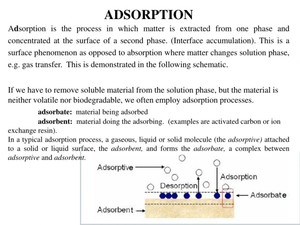
Measuring Adsorption Adsorption defined as surface excess with respect to bulk soil solution mqi = ni - VCi where qi is moles of species i per unit mass of adsorbent ni is total moles of species i in the system ci is solution concentration of species i m is mass of adsorbent V is solution volume Batch and flow methods for determining In either, reaction time should be long enough to allow accumulation of adsorbate but short enough to avoid side reactions like precipitation / dissolution, redox or degradation
Example Soil / solution suspension consisting of 0.010 kg soil and 0.040 L water contains a total of 0.005 mol Ca and has a [Ca] = 0.040 M q = (n – VC) / m q = (0.005 mol – 0.040 L x 0.040 M) / 0.010 kg = 0.34 mol kg-1 Soil / solution suspension consisting of 0.010 kg soil and 0.040 L water contains a total of 0.010 mol Cl and has a [Cl] = 0.300 M q = (0.010 mol – 0.040 L x 0.300 M) / 0.010 kg = -0.20 mol kg-1 Commonly, adsorption determined from change in solution concentration qi = V(C0 - Ci)
Of course, one is never quite sure that a change in solution concentration is, in fact, due to adsorption Semi-proof would come from knowledge of mineralogical composition of soil, together with spectroscopic data for reaction product(s) given by pure mineral(s)
Adsorption Equilibria Equilibrium is not instantaneous in any case but often effectively instantaneous Recall earlier example of cation adsorption in which approach to equilibrium was limited only by diffusion But for specific adsorption (with inner-sphere surface complex formation), approach to equilibrium is much slower If instantaneous equilibrium does not occur, general kinetic expression applicable, dCi / dt = Rf - Rr Otherwise, isotherms, qi = F(ci), for constant T and P used to describe the partition of species i between adsorbed and solution phases
General types, S, L, H and C Isotherms S curves have initially small slope that increases with increasing adsorptive concentration Possible explanations include Solution phase complexation of the adsorptive as with complexation of dissolved Cu by dissolved organic matter (high affinity for complexation) Once capacity of dissolved organic matter to complex Cu reached, adsorption proceeds Cooperative interactions of the adsorbed species Increasing extent of adsorption leads to increased affinity for adsorption
L curves have initially steep but decreasing slope with increasing concentration of the adsorptive Shape due to initially high affinity but decreasing area (number of sites) for continued adsorption as the extent of adsorption increases Langmuir and Freundlich are example models S = kSMC / (1 + kC) S = kCN Langmuir can be developed from above concept that extent of adsorption is proportional to the concentration of adsorptive, C, but decreases with extent of adsorption dS / dt = kfC(SM – S) - krS
Langmuir can be used in conjunction with a site affinity distribution function to derive other isotherms qi / Qi = ∫ (Ck(x) / (1 + Ck(x)) G(x) dx where G(x) is the site affinity distribution function H curve is exaggerated form of L Often due to inner-sphere surface complex formation C curve has constant slope, with neither increasing (S curve) nor decreasing (L or H curves) slope with increasing concentration of the adsorptive
Metal Cation Adsorption Strength of adsorption Inner-sphere > Outer-sphere > Diffuse ion swarm Inner-sphere, electronic structure of surface functional group and metal cation control adsorption Outer-sphere complexation, similar to inner-sphere but smeared-out surface charge and cation valence partly control Diffuse ion swarm affected only by surface charge and valence
Inner-sphere complexation For constant Z, tendency increases as ionic potential, Z / r, decreases Small Z / r (large r) species will lose hydration water (easier to de-solvate) and form inner-sphere complex with surface functional group Small Z / r (large r) species more easily polarized by electronic field of surface functional group, leading to ~covalent bonding Cs+ > Rb+ > K+ > Na+ > Li+ Ba2+ > Sr2+ > Ca2+ > Mg2+ But trend for transitional metals Cu2+ > Ni2+ > Co2+ > Fe2+ > Mn2+ more difficult to account for
pH effects on metal cation adsorption Via surface charge, σH (pH increases, σH becomes more -) Adsorption edge, qi = F(pH) Generally, if high pH is necessary for adsorption, affinity low pH50 pH50Na > pH50Cs but adsorption Na+ < Cs+ Since hydrolyzed species are more easily de-solvated, if appreciable hydrolysis occurs below pH50, M(OH)n(m-n)+ is involved in adsorption process
Role of complexing ligands in solution M(ad) ML(ad) L(ad)
Anion Adsorption Inner-sphere > outer-sphere > diffuse ion swarm Among common anions in soil solution, B(OH)4-, (H2PO4-, HPO42- and PO43-) and COO- tend to form inner-sphere Cl-, NO3- and, to some extent, HCO3-, CO32- and SO42-, outer-sphere or to be adsorbed in the diffuse ion swarm
Inner-sphere complexation Involves ligand exchange of the anion for either surface bound water (protonated hydroxyl) or hydroxyl SOH + H+ SOH2+ SOH2+ + Ll- SL(l-1)- + H2O or SOH + Ll- SL(l-1)- + OH- Favored by pH < PZNPC, however, persists beyond Evidence from spectroscopic and pH measurements
Outer-sphere SOH2+ + Ll- SOH2+Ll- SMm+ + Ll- SMm+Ll- In either case, ligand is hydrated so that there is no direct contact Evidence that anions like Cl- are either adsorbed as outer-sphere complexes or in the diffuse ion swarm These species are readily displaced (exchanged) Adsorption substantially decreases as PZNPC approached May exhibit negative adsorption
Adsorption (mol / kg) qi = (1/ms) [ci(x) –c0i] dV which may be negative as in the previous example Soil / solution suspension consisting of 0.010 kg soil and 0.040 L water contains a total of 0.010 mol Cl and has a [Cl] = 0.300 M q = (0.010 mol – 0.040 L x 0.300 M) / 0.010 kg = -0.20 mol kg-1 An exclusion volume can also be calculated, VEX = [(1/ms) [ci(x) – c0i] dV] / c0i = -qi / c0i, which for this example would be VEX = -0.20 mol kg-1 / 0.300 M = -0.667 L kg-1 VEX / VH2O = 0.667 / 4 = 0.167 so peak BTC of pulse at 0.833 PV
pH effects on anion adsorption Via surface charge, σH (pH decreases, σH becomes less -) • favored at pH < ZPNPC However, for an anion that becomes protonated, this effect is offset -at low pH protonation of the adsorptive renders it non-adsorbed Adsorption envelope, qi = F(pH)
Compare adsorption envelopes for monoprotic and di- / triprotic anions
Molecular Adsorption Models Gouy-Chapman (Diffuse Double Layer) Stern Modification Constant Capacitance Models
Gouy-Chapman • For space normal to a planar charged surface and non-interacting point charges • in solution with only two species of same valance, c+ and c- • 1. Beginning by equating electrochemical potentials of a species in the • diffuse ion swarm and bulk solution, derive the Boltzmann distribution relating • concentration, c+/- at any position x to the electric potential at x, Ψ(x), • c+(x) = c+0 exp(-z+Ψ(x) / RT) • c-(x) = c-0 exp(z-Ψ(x) / RT) • Relate charge density, ρ(x) = ΣciziF, to potential using the Poisson equation • for this one-dimensional space, • d2Ψ / dx2 = F(ρ) = G(c+(x), c-(x)) • and solve this equation to find the relationship, Ψ = H(x)
More explicitly, d2Ψ / dx2 = -4πρ / ε = -(4π / ε) zFc0 [exp(-zFΨ / RT) – exp(zFΨ / RT)] Derivations combine parameters to simplify operations but arrive at (dΨ / dx) d (dΨ / dx) = -(4π / ε) zFc0 [exp(-zFΨ / RT) – exp(zFΨ / RT)] dΨ which is integrated to (dΨ / dx)2 = (8π / ε) RT c0 [exp(-zFΨ / RT) + exp(zFΨ / RT)] + B or dΨ / dx = -{(8π / ε) RT c0 [exp(-zFΨ / RT) + exp(zFΨ / RT) – 2]}1/2 where B = - 2 (8π / ε) RT c0 since if x is large, both dΨ / dx and Ψ are 0 This is the same as Sposito Eq. 8.16 if the exponentials were expressed as concentrations as per Boltzman and since 4π / ε = 1 / ε0D
This expression is then integrated, i.e., dΨ / {(8π / ε) RT c0 [exp(-zFΨ / RT) + exp(zFΨ / RT) + 2]} = -dx using hyperbolic identities to simplify the matter and a constant of integration is determined as zFΨ0 / RT at x = 0. But to obtain an explicit dependence of Ψ on x, more identities are needed to finally arrive at, Ψ = (2RT / zF) ln [exp(κx) + tanh(zFΨ0 / 4RT)] – (2RT / zF) ln [exp(κx) - tanh(zFΨ0 / 4RT)] where κ = 8πz2F2c0 / εRT
This establishes c+/- (x) • c+(x) = c+0 exp(-z+Ψ(x) / RT) • c-(x) = c-0 exp(z-Ψ(x) / RT) • Surface charge density, σ, is found by integrating ρ(x) from the surface • outward, since σ is equal but opposite to this integral • σ = - ρ(x) dx • where ρ(x) = - (ε / 4π) d2Ψ / dx2 and the integration is from the surface to • a distance far away. This gives • σ = -(ε / 4π) (dΨ / dx) at the surface, since far away dΨ / dx = 0. • From previously, • dΨ / dx = -{(8π / ε) RT c0 [exp(-zFΨ0 / RT) + exp(zFΨ0 / RT) – 2]}1/2
So that σ = (ε / 4π) {(8π / ε) RT c0 [exp(-zFΨ0 / RT) + exp(zFΨ0 / RT) – 2]}1/2 σ = {(ε RT c0 / 2π) [exp(-zFΨ0 / RT) + exp(zFΨ0 / RT) – 2]}1/2 which is the same as Sposito 8.17 since ε / 2π = 2 / ε0D, except for the coefficient S / F. σ is charge per unit area here. Multiplying by S / F (m2 kg-1 / C mol-1) converts units of σ to mol (+/-) kg-1 as used in Chapter 7.
Stern Modification Accounts for specific adsorption of finite-size ions (not point charges) Application to Variable Surface Charge Soils
Stern Modification Allows for surface adsorption, beyond which exists the diffuse layer of ions. σ = σS + σD σS = NizF / [1 + (NAρw / Mwc) exp(-(zFΨd + Φ) / RT)] where Ni is number of adsorption sites per area ρ is density of water Mw is mass of water Ψd is potential at the thickness of the Stern layer, d Φ is specific adsorption potential σD is as before but with Ψd
Application to Variable Surface Charge Soils Unlike the Gouy-Chapman (double layer) system in which the surface charge is constant, surface charge variability arises due to adsorption / desorption of H+ relative zero surface charge. As with Gouy-Chapman, σ = {(ε RT c0 / 2π) [exp(-zFΨ0 / RT) + exp(zFΨ0 / RT) – 2]}1/2 but Ψ0 = (RT / F) ln (H+) / (H+0) where (H+0) is that for Ψ0 = 0 Thus, σ = {(ε RT c0 / 2π) [(H+0)z / (H+)z + (H+)z / (H+0)z – 2]}1/2 σ = {(ε RT c0 / 2π) [10-z(pH0 – pH) + 10z(pH0-pH) – 2]}1/2
Surface Complexation Consider the surface complexation reaction SO-(s) + Cu2+(aq) = SOCu+(s) K = (SOCu+) / (SO-) (Cu2+) however, what can be measured is cK = [SOCu+] / [SO-] (Cu2+) which varies with [SOCu+] and [SO-] This approach models surface phase activity as (SOCu+) = [SOCu+] exp(zFΨo / RT) and (SO-) = [SO-] exp(-zFΨo / RT) where z = 1 in this case
So K = [SOCu+] exp(zFΨo / RT) / [SO-] exp(-zFΨo / RT) (Cu2+) or K = cK exp(2zFΨo / RT) The constant capacitance model assumes that σP = SCΨo / F K = cK exp(2zF2σP / SCRT) σP = σ0 + σIS = σ0 + 2[SOCu+] But the permanent charge is -([SO-] + [SOCu+]) so σP = -[SO-] + [SOCu+]
If in a solution of Ca2+ and Cl- there is an adsorbent with non-protonated • SOH sites, and sites SOH2+, SO-, SOCa+, and SOH2+Cl-, where each • refers to a mole of such sites, define σH, σIS, σOS and σD in terms of • concentrations of the surface species, i.e, [SOH2+] etc. The surface • complex SOCa+ is inner-sphere. • σH = qH - qOH = [SOH2+] + [SOH2+Cl-] – [SO-] – [SOCa+] • σIS = 2[SOCa+] • σOS = - [SOH2+Cl-] • Since, σD = -(σH + σIS + σOS), assuming σ0 = 0 • σD = -[SOH2+] - [SOCa+] + [SO-]
A variably charged soil contains 0.40 μmol SOHTotal / m2 and 0.25 μmol SOH2+ / m2. If F- is adsorbed at pH < ZPNPC, show that the molar ratio of adsorbed H+ to adsorbed F- is ~ 0.6. qH = 0.25 μmol m-2 so qOH = 0.0 to 0.15 μmol m-2 Assuming adsorption at all possible sites, qF = 0.25 to 0.40 μmol m-2 (qH / qF) = (0.25 / 0.40) to (0.25 / 0.25) or 0.625 to 1 Unlikely that no SOH sites exist, i.e., likely that qOH > 0 so that (qH / qF) = 0.625 to < 1 Also, adsorption of F- by displacement of OH- or H2O raises the pH which reduces qH and increases qOH. The latter limits qF to < 0.40.


![protein adsorption [%]](https://cdn3.slideserve.com/5518059/slide1-dt.jpg)