Download
1 / 44
600 likes | 1.23k Views
LR Phono Preamps. Pete Millett ETF.13 pmillett@hotmail.com. Agenda. A bit about me Part 1: What is, and why use, RIAA? Grooves on records The RIAA standard Implementations of RIAA EQ networks and preamps Testing phono preamps Part 2: Implementing LR RIAA equalization

E N D
LR Phono Preamps Pete Millett ETF.13 pmillett@hotmail.com
Agenda • A bit about me • Part 1: What is, and why use, RIAA? • Grooves on records • The RIAA standard • Implementations of RIAA EQ networks and preamps • Testing phono preamps • Part 2: Implementing LR RIAA equalization • Example preamp circuits • Problems: Inductor imperfections • Working around the problems NOT a discussion about why one would use LR, or if it sounds better than RC!
A bit about me • I live near Dallas, Texas, USA • But I’m not really a Texan! • Worked as an EE for over 30 years • Mostly board-level computer & computer peripherals • Lately mostly doing integrated circuit product definition • Have a “hobby business” building high-end headphone amps and DIY PC boards for tube audio projects
Part 1: RIAA What is RIAA, anyway? And why do we need it?
Grooves on a record – the basics • Sound is recorded on a record by cutting a groove that wiggles according to the amplitude of the recoded signal • To play the record, we use a stylus that moves with the groove • The cartridge typically uses a magnet and a coil, one of which moves with the stylus. The movement of the magnetic field through the coil generates a small voltage.
Grooves on a record – stereo • Stereo recording is done with two magnets and coils at a 90 degree angle from one another
Playback - phono cartridges • Modern phono cartridges fall into two main groups: moving coil (MC), and moving magnet (MM) • MC cartridges have a stationary magnet, and the coil moves with the stylus. MM cartridges are the inverse, with a magnet moving with the stylus and fixed coils. • In a MC cartridge, the coils are very small, so MC cartridges typically have very low output voltage • Typically about 60dB of gain @ 1kHz is needed for MC cartridges - 40-45dB is needed for a MM cartridge.
Groove geometry vs. frequency • The amplitude of the signal produced by moving a magnetic field through a coil is proportional to the velocity of the motion • To get the same amplitude out of a phono cartridge at all frequencies, the groove would need to be very wide at low frequencies, and very tiny at high frequencies • This would limit the amount of material that could be recorded on a disk (because of the large swing at LF), and generate lots of HF noise (because of the tiny swing at HF) • What to do?
Phono equalization (EQ) • One could use a constant-amplitude recording method, which makes the record groove the same physical size at all frequencies • To do this, the voltage applied to the cutting head must increase with frequency… then the output of a playback cartridge will decrease with frequency • Playback requires equalization, attenuating the signal with frequency, to get flat reproduction of the original signal • Constant-amplitude recording has problems: at low frequencies, the large playback gain amplifies LF noise like turntable rumble. And at high frequencies, the cutter velocity becomes very high. • A better solution is to combine regions of constant-velocity recording with regions of constant-amplitude recording • RCA introduced the “New Orthophonic” curve in 1953 that did just that • This is what became the RIAA standard in 1956 that we use today
The RIAA EQ standard • The standard set by the RIAA defines the EQ curve to be used on records • The recording EQ curve is flat to 50Hz, then increasing amplitude to 500Hz, flat to 2120Hz, then increasing • The playback EQ curve is the inverse of this. It has a pole (low-pass characteristic) at 50Hz, a zero (high-pass) at 500Hz, and another pole at 2122Hz. • The poles and zeros are also referred to by their time constants of 3180µS, 318µS, and 75µS. The frequency is found by f = 1/(2*p*t) pole Recording pole zero Playback
Poles and zeros using capacitors • A pole or zero can be created by a resistor, and a reactive component - either a capacitor… f(-3dB) = 1 / (2* p * R * C)
Poles and zeros using inductors …or an inductor f(-3dB) = R / (2 * p * L)
RIAA preamp implementations • Phono preamps can be implemented several ways: • “Passive” preamps put the EQ section in series with the signal • “Active” preamps put the EQ in a feedback network around an amplifier • A combination of active and passive is also possible Passive Active Amp Amp In Amp EQ + In Out Out - EQ • The EQ function can be performed by any combination of inductors, capacitors, and resistors. • The amplifier sections can be any combination of opamps, vacuum tubes, or transistors
Passive RIAA EQ networks • Many other permutations are possible • In reality, it’s not this straightforward. The nonzero source impedance of each stage interacts with the following stage.
Passive RIAA example • Below is an example of a phono stage with passive RC EQ (RCA tube manual) with the RIAA EQ highlighted
Active RIAA tube circuit example • Below is an example of an phono stage with an active EQ (Dynaco PAS preamp)
More RIAA examples • These circuits are from Walt Jung’s “Signal Amplifiers” • Note the two possible transpositions of EQ components (“N1” and “N2” networks)
How to test RIAA preamps? • To test and measure an RIAA phono preamp, one could just apply a voltage to the input, vary the frequency, and measure the output • But the small signals involved make this a little difficult • The best approach is to use an “inverse RIAA” network. This simulates the output of a cartridge, so the measured output of the preamp should be flat • I used one made my Hagerman Technology - www.hagtech.com/iriaa2.html • It’s accurate to within +/-0.4dB and has convenient 40dB and 60dB attenuation
Part 2: LR RIAA equalizers How to implement LR RIAA? And avoid some problems…
LR EQ: passive or active • An LR EQ can be implemented in series with the signal, or in the feedback loop of the amplifier • I looked at active LR EQ (in the feedback loop of an opamp), but soon discovered that inductor imperfections made it very difficult to create a stable design • Has anybody succeeded in building an active LR EQ?
A tube LR RIAA preamp • This is Steve Bench’s design from 2004 • Note R4, which (I think) is adding a zero to compensate for the transformer response, and maybe something else too (more later)
An opamp-based LR RIAA preamp • Here is my initial design of a passive LR preamp: • The first stage has a gain of 20dB; the second, 41dB • L1 and R2 form the 50Hz pole, L1 and R3 the 500Hz zero, and L5 and R4 form the 2200Hz pole • The EQ attenuates about 21dB @ 1kHz, so the net gain is 40dB @ 1kHz • Exact resistor values were derived from simulation, since there is some interaction between the stages
Circuit simulation: passive LR EQ • If we simulate my circuit using an inverse RIAA network at the input, it looks very good: within 1/2dB 20Hz – 20kHz!
Circuit measurement: passive LR EQ • If we build and measure this circuit, it looks OK, but not as good: still down less than 3dB at 20kHz. One could live with this…
High frequency response • HOWEVER…. What if we look out to 100kHz? • What is this?
Inductor imperfections (parasitics) • Unfortunately, a real inductor is not just an inductor. It has parasitic resistance (the resistance of the wire), parasitic capacitance, and other non-ideal characteristics. • The resistance can be modeled as a resistor in series with the inductor; capacitance can be (roughly) modeled as a capacitor in parallel:
Impedance of an ideal inductor • An ideal inductor has an impedance that varies linearly with frequency, equal to the inductive reactance, which is 2 * p * f * L • So the impedance of an ideal inductor (1mH) is a straight line:
Impedance of a real inductor • …but add 50pF of parasitic capacitance and it looks like this:
Self-resonance • This effect of the parasitic shunt capacitance is called “self-resonance”. The inductor and its parasitic capacitance form a parallel resonant circuit, which has a very high impedance at the resonant frequency • Generally, the higher the inductance, the lower the SRF (Self Resonant Frequency), since there are more turns of wire in a larger inductor • In a passive LR EQ network, self-resonance causes a notch in frequency response at the SRF, because the impedance is very high there… • …followed by a increase in gain, because above the SRF, the inductor is now effectively a capacitor, with decreasing impedance with frequency!
Measurement of a real inductor • I measured the inductor I used, a 520mH pot core part from Cinemag, using a 1k series resistor • You can see the LR pole formed by the inductor and the 1k resistor, located at about 300Hz. • At ~40kHz, there is a notch – this is self-resonance • Above self resonance, the response climbs back to zero dB
Modeling the real inductor • An ohmmeter and a little trial and error in pSpice tells us what the parasitics of this inductor are • The simulation looks exactly like the measurement • f(SRF) = 1 / (2 * p * L * C )
Fixing the inductor • There are ways to build inductors with less parasitic capacitance, so a higher SRF • This typically involves special winding geometries, sectioned windings, insulating layers, or magic! • They can cause the inductor to be physically larger, and more expensive, and certainly harder to build • There are transformer winders here that can explain more! • An example of a winding method used to increase SRF is the RF choke – the windings are separated into sections to break up the interwinding capacitances, which gives you a higher frequency SRF than a solenoid-wound coil
Self-resonance in my circuit Since the SRF of a larger inductor is typically lower than that of a smaller one, you may think that the larger inductor in my design would be the problem here However, I used the same inductor in both locations. The inductor is tapped – I use the full winding for the 50Hz pole and only a part of it for the 2122Hz pole. But the rest of the coil is still there, so its SRF is not lower than if I used the entire winding – still 40kHz. Same SRF
Avoiding the SRF with a zero • There is a barely perceptible dip at the SRF, but no notch! • At the SRF, the resistor dominates • So in an LR EQ, the SRF can be avoided… sometimes… • See what happens when we add a zero below the SRF:
Working around the self-resonance Because my first L has a zero (parallel R), the second inductor SRF is causing the notch and gain rise here If we add a resistor (R1 below) across the other inductor and create another zero just below the SRF of the inductor, we can remove the notch Tuning is critical The HF peak is still there, rising until ~400kHz
The HF peak • We don’t want too much excessive gain above the audio frequencies, to prevent amplification of unwanted signals (like an AM radio station!) • Ultrasonic gain can be lowered by adding a high-frequency pole to the system. A small inductor is used, with a very high SRF.
A (mostly) complete simulation • Still an HF peak at ~400kHz, but its reduced from ~33dB to ~14dB • A small drop at LF due to the resistance of the new inductor
Final measurement • The response of the preamp after these changes is within +/-1dB 20Hz – 20kHz • Channels track within +/- 0.3dB
Final measurement • Still a rising response above 50kHz • Peak is only +2.2dB @ 240kHz… better than simulation
Questions? Still awake? Thanks!