Symmetry breaking instabilities in granular gases. Lectures I and II.

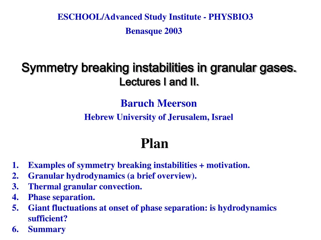
1. ESCHOOL/Advanced Study Institute - PHYSBIO3 Benasque 2003 Symmetry breaking instabilities in granular gases.Lectures I and II. Baruch Meerson Hebrew University of Jerusalem, Israel Plan • Examples of symmetry breaking instabilities + motivation. • Granular hydrodynamics (a brief overview). • Thermal granular convection. • Phase separation. • Giant fluctuations at onset of phase separation: is hydrodynamics sufficient? • Summary

2. A few pictures of the Hebrew University of Jerusalem

3. A few pictures of Jerusalem

4. Example 1. Granular Maxwell’s Demon: phase separation by symmetry breaking Schlichting and Nordmeier (1996), Eggers (1999), Lohse et al. (2001), Brey et al. (2002),… theory original experiment more experiment + theory

5. Granular Maxwell’s Demon (continued): coarsening Lohse et al. (2002) Coarsening will be considered in Lecture 3.

6. Example 2. Phase separation (and coarsening) by symmetry breaking in a granular monolayer driven by vertical vibrations Experiment: Olafsen and Urbach (1998) MD simulations: Nie et al. (2000), Cafiero et al. (2000) static (crystalline) cluster “gas”

7. Before going further: Gas of Inelastic Hard Spheres s: particle diameter m: particle mass inelastic binarycollisions (simplest model) coefficient of normal restitution: coefficient of normal restitution

8. In most cases, this model cannot describe granular solids: It does describe many aspects of granular liquids: and, of course, granular gas.

9. Example 3. “Thermal” granular convection Inelastic particle collisions cause a negative temperature gradient g Driving wall MD simulations:Ramìrez et al. (2000), Sunthar and Kumaran (2001). Experiment:Wildman et al. (2001,2002). Theory: He, M. and Doolen (2002), Khain and M. (2003)

10. Example 4. Clustering in a freely cooling granular gas density map Luding (2002) Goldhirsch and Zanetti (1993) Strongly inelastic collisions, narrow cluster bands (few particle diameters) Nearly elastic collisions, 1-r<<1 muchwider cluster bands: Granular Hydrodynamics has better chances to be valid

11. Motivation: why should we care about symmetry breaking instabilities (SBIs)? • SBIs provide sensitive tests to models of granular flows • They improve our understanding of pattern formation far from equilibrium • They are cool

12. II. Navier-Stokes granular hydrodynamics (GH): an overview GH operates with three coarse-grained fields: r (r,t): granular density v(r,t): granular velocity T(r,t): granular temperature a compressible fluid! Formal definitions: n(r,t): local number density Averaging over cells that are small compared to the system size, but still include many particles

13. Equations of Navier-Stokes GH mass conservation P: stress tensor Q: heat flux G:rate of energy loss by collisions per unit volume f: external force momentum conservation energy equation d=2 or 3: dimension of space More fundamental kinetic theory validates these equations and supplies constitutive relations:Jenkins and Richman, Tan and Goldhirsch, Brey et al.

14. “Standard” constitutive relations of GH Jenkins and Richman (1985,1988) rate of deformation tensor deviatoric part of D G, F, J and M:functions ofnps 2(d=2), or nps 3(d=3) a1, a2, a3, a4anda5,:numbers Conveniently presented by Babić (1993) Valid for nearly elastic collisions, 1-r<<1,and at small or moderate densities

15. The energy sink term G: asimple estimate Energy lost in each collision: A particle with speed vT~ (T/m)1/2 loses, on the average, energy ~m (1-r2) vT2. Collision rate ~vT/l, where l is the mean free path. n particles in unit volume. d=2, dilute limit

16. When is the Navier-Stokes GH valid? • Not a simple question. Important necessary conditions are: • Mean free path and particle diameter are small compared to any length scale described hydrodynamically. • Mean time between two consecutive collisions are small compared to any time scale described hydrodynamically. • Only single, liquid-like phase. • Velocity distribution function f(v,r,t) is “close to Maxwellian” at all r and t of interest. • Inelastic collapse doesn’t happen (or removed by a regularization). 1,2,4 and 5 are usually satisfied for nearly elastic collisions, 1-r<<1 (quite a restrictive condition! OK for glass balls, steel balls.) 3 is expected to break down at high densities. In general, this requires introduction of an order parameter into theory, cf.Aranson and Tsimring (2002), even for the hard sphere model. Sometimes, condition 3 can be relaxed:Grossman et al. (1997), M., Pöschel and Bromberg (2003), Gollub et al… Not always clear why.

17. Checking GH in MD simulations of a simple steady state thermal wall M., Pöschel, Sasorov and Schwager (2002) Works well Many other systems checked. No major disagreements found when conditions 1-5 are met (one open question is still under investigation, wait for the end of Lecture II). Boundary conditions may introduce additional limitations, if one wants to have a full hydrodynamic problem.

18. Relaxing condition 3: close-packed “floating”cluster MD simulations experiment Lohse et al. (2003) M., Pöschel and Bromberg (2003)

19. A simple version of Granular Hydrostatics [Grossman, Zhou and Ben-Naim (1997)]works well at all densities, up to hexagonalclose packing g T=const Phase coexistence doesn’t seem to play a big role here M., Pöschel and Bromberg (2003)

20. g H III. Back to thermal granular convection T0 Governing equations in the dilute limit stress tensor Froude number (may go to infinity) Governing parameters: Knudsen number Relative heat loss parameter He, M. and Doolen (2002)

21. Basic state: no mean flow • may show a density inversion Solvable analytically r T “Thermal” wall at y=0 y T goes down with the height y: Inelastic collisions cause a negative temperature gradient

22. Linear stability analysis of the trivial state Khain and M. (2002) Fourier analysis in x direction Linearization of equations, numerical solution. Marginal (or neutral) stability condition: g=0 0.9 unstable like in Rayleigh-Benard convection 0.8 R*c 0.7 1 2 3 R > R*c (F,K) convection

23. 3 Dependence of the threshold on the Froude number 2 Phase separation instability 1 0 2 4 F>>1 drops out: localization of granulate near base Large-F limit Convection cells at onset

24. Schwarzschild’s criterion for classical convection in compressible fluid S: entropy of fluid no convection

25. Schwarzschild’s criterion works for granular convection: Define entropy S(r,T) like in classic case (r=1) convection threshold 3 Schwarzschild’s criterion 2 1 0 1 2 3 4

26. Convection threshold versus Knudsen number K viscosity suppress convection heat conduction 1.5 1 0.5 0 0 0.02 0.04 Schwarzschild’s value

27. Hydrodynamic simulations of thermal granular convection: solving full hydrodynamic equations numerically He, M. and Doolen (2002) Supercritical bifurcation, in agreement with MD simulations by Ramìrez et al. (2000) Next (huge) step: developing a weakly nonlinear theory close to onset. Can Boussinesque approximation be validated?

28. IV. Phase-separation instability “hot” wall Model: elastic wall stripe state gravity = 0 Steady state obeys: 0.4 r “hot” wall 0.3 T elastic wall 0.2 0.1 0 0 0.2 0.4 0.6 0.8 1 X Early work: Theory: Grossman et al. (1997).Experiment: Kudrolli et al. (1997)

29. heat conduction heat loss GH predicts instability of the stripe state, 2D steady states appear. Livne, M. and Sasorov (2000,2002), Khain and M.(2002) Steady-state describable by hydrostatic equations: Stripe state: 1D solution of these eqns. multiple hydrostatic solutions possible, stripe can be unstable or metastable nonlinearproblem

30. Governing parameters of the hydrostatic equations hydrodynamic heat loss parameter area fraction aspect ratio Livne, M. and Sasorov (2000,2002); Khain and M. (2002)

31. Physics of stripe state L>LC p Negative compressibility! f p(f,L): steady-state pressure of stripe state Khain and M. (2002), Argentina et al. (2002)

32. Spinodal interval 0.05 p L<LC 0.04 L=LC spinodal interval 0.03 0.02 L>LC 0.01 f 0 0 0.06 0.12 0.18 everywhere L<LC LC: Argentina et al. (2002), KMS critical point Stripe state unstable within spinodal interval Infinite layer

33. Analogy: P-V isotherms of van der Waals gas Spinodal region Coexistence region

34. What if D is finite? L>LC P Negative compressibility Negative lateral compressibility:destabilizing effect f Lateral heat conduction: stabilizing effect Critical lateral length: D > Dc for instability

35. How to find Dc , the critical lateral length for instability? Marginal stability analysis Close to continuous bifurcation threshold scaled inverse density Yk is small linearization of hydrostatic eqns. Schrödinger equation for k(x) k: discrete energy level KM 2002

36. Dc at different  k/1/2 f k: wave number along stripe Stripe stable beyond curve D > Dc=p/kcandf1<f<f2 needed for instability LMS (2000,2002); KM (2002), Brey et al. (2002)

37. Bifurcated state (droplet) above critical value of D close-packed droplet Δ=1.3 color density maps Δ=3 Δ=1.2 c= 1.28 =12,500 f=0.0378 LMS 2002

38. Coarsening dynamics: hydrodynamic simulations Gas-mediated coarsening Λ=12,500 f=0.0378 Δ=6 Hydro simulations used Stokes friction instead of full viscosity LMS 2002 Final state: one close-packed droplet

39. Direct mergers of clusters also happen Λ=12,500 f=0.0378 Δ=6 Same final state! LMS 2002

40. 0 1 2 3 5 6 7 4 Supercriticalbifurcation diagram: theory vs. (overdamped) hydrodynamic simulationsYc: normalized y-coordinate of center of mass 0.5 theory 0.4 Yc 0.3 0.2 =12,500 f=0.0378 0.1 D Δc  1.28 Excellent agreement with analytic theory not too far from threshold

41. MD simulations(M, Pöschel, Sasorov and Schwager 2002) N=2·104 D << Dc Δc = 0.5 Δ= 0.1 weakly fluctuatingstripe state, hydrostatics (and overdamped hydrodynamics) are doing well

42. D> Dc MD simulations hydro simulations MPSS (2002) LMS (2002) N=2·104 Nucleation, coarsening of droplets, one droplet survives. Hydrostatics (and overdamped HD) are doing well.

43. Very large aspect ratio:D>> Dc MD simulations Argentina et al. (2002) fluctuations weak, hydrostatics OK Outside of spinodal interval, inside coexistence interval

44. What happens around D ~ Dc?MD simulations N=2·104 Transitions between the two states with broken symmetry?

45. Center-of-mass dynamics Giant fluctuations Hydrostatics fails in awideregion around Dc

46. Probability distribution of Yc at different D Symmetry-breaking transition occurs somewhere at 0.3 < D < 1,hydrostatics predicts Dc = 0.5.

47. Probability distribution maxima vs. D hydro simulation hydrostatic bifurcation curve maxima of PDF Systematic disagreement with hydrostatics within fluctuation-dominated region. Change of bifurcation character?

48. What is so unusual here? Fluctuation regionanomalouslywide For comparison:transition to convection (when one adds gravity) doesn’t show any “noise anomaly”: N=2,300 MD simulations: Ramirez et al. (2000), Hydrodynamics: HMD (2002), KM (2003) Where do the giant fluctuations come from?

49. Yc vs. N at fixed L, f and D<Dc N=20000 N=15000 N=10000 N=5000 Low-frequency oscillations don’t seem to go down as N increases

50. Scenario I. Giant fluctuations are driven hydrodynamically: by a (yet unknown) instability (Ia), or by a long-lived transient (Ib) To check this scenario, one needs full hydrodynamic simulations (Livne, M. and Sasorov; work in progress).