CSE 190D Database System Implementation

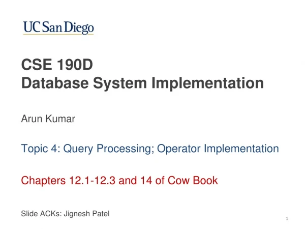
Topic 4: Query Processing; Operator Implementation Chapters 12.1-12.3 and 14 of Cow Book CSE 190DDatabase System Implementation Arun Kumar Slide ACKs: Jignesh Patel

|…|……|………..|………..| |…|……|………..|………..| |…|……|………..|………..| |…|……|………..|………..| |…|……|………..|………..| |…|……|………..|………..| |…|……|………..|………..| |…|……|………..|………..| |…|……|………..|………..| |…|……|………..|………..| |…|……|………..|………..| Query Scheduler Execute Operators Select R.text from Report R, Weather W where W.image.rain() and W.city = R.city and W.date = R.date and R.text. matches(“insurance claims”) Optimizer Parser Lifecycle of a Query Query Query Result Physical Query Plan Segments Syntax Tree and Logical Query Plan Query Result Query Database Server

Recall the Netflix Schema Ratings Users Movies

Example SQL Query SELECT M.Year, COUNT(*) AS NumBest FROM Ratings R, Movies M WHERE R.MID = M.MID AND R.Stars = 5 GROUP BYM.Year ORDER BYNumBest DESC Suppose, we also have a B+Tree Index on Ratings (Stars)

Result Table SELECT R.stars = 5 SELECT No predicate SORT On NumBest JOIN R.MID = M.MID GROUP BY AGGREGATE M.Year, COUNT(*) Logical Query Plan Ratings Table Movies Table Called “Logical” Operators From extended RA Each one has alternate “physical” implementations

Result Table Physical Query Plan File Scan Read heapfile Index-Nested Loop Join Hash-based Aggregate Indexed Access Use Index on Stars External Merge-Sort In-mem quicksort; B=50 Ratings Table Movies Table Called “Physical” Operators Specifies exact algorithm/code to run for each logical operator, with all parameters (if any) This is one of many physical plans possible for a query!

Logical-Physical Separation in DBMSs Logical = Tells you “what” is computed Physical = Tells you “how” it is computed Declarativity! Declarative “querying” (logical-physical separation) is a key system design principle from the RDBMS world: Declarativity often helps improve user productivity Enables behind-the-scenes performance optimizations People are still (re)discovering the importance of this key system design principle in diverse contexts… (MapReduce/Hadoop, networking, file system checkers, interactive data-vis, graph systems, large-scale ML, etc.)

Operator Implementations Select Project Join Set Operations Group By Aggregate Need scalability to larger-than-memory (on-disk) datasets and high performance at scale!

But first, what metadata does the RDBMS have?

System Catalog • Set of pre-defined relations for metadata about DB (schema) • For each Relation: • Relation name, File name • File structure (heap file vs. clustered B+ tree, etc.) • Attribute names and types; Integrity constraints; Indexes • For each Index: • Index name, Structure (B+ tree vs. hash, etc.); IndexKey • For each View: • View name, and View definition

Statistics in the System Catalog • RDBMS periodically collects stats about DB (instance) • For each Table R: • Cardinality, i.e., number of tuples, NTuples (R) • Size, i.e., number of pages, NPages (R), or just NR or N • For each Index X: • Cardinality, i.e., number of distinct keys IKeys (X) • Size, i.e., number of pages IPages (X) (for a B+ tree, this • is the number of leaf pages only) • Height (for tree indexes) IHeight (X) • Min and max keys in index ILow (X), IHigh (X)

Selection: Access Path • Access path: how exactly is a table read (“accessed”) • Two common access paths: • File scan: • Read the heap/sorted file; apply SelectCondition • I/O cost: O(N) • Indexed: • Use an index that matches the SelectCondition • I/O cost: Depends! For equality check, O(1) for hash index, and O(log(N)) for B+-tree index

Indexed Access Path R

Selectivity of a Predicate • Selectivity of SelectionCondition = percentage of number of tuples in R satisfying it (in practice, count pages, not tuples) R Selectivity = 2/7 ~ 28% Selectivity = 3/7 ~ 43% Selectivity = 1/7 ~ 14%

Selectivity and Matching Indexes • An Index matches a predicate if it brings I/O cost very close to (N * predicate’s selectivity); compare to file scan! R N x Selectivity = 2 Hash index on R(Stars) Cl. B+ tree on R(Stars) Uncl. B+ tree on R(Stars)? Assume only one tuple per page

Matching an Index: More Examples R Hash index on R(Stars) does not match! Why? Cl. B+ tree on R(Stars) still matches it! Why? Cl. B+ tree on R(Stars,RateDate)? Cl. B+ tree on R(Stars,RateDate,MID)? Cl. B+ tree on R(RateDate,Stars)? Uncl. B+ tree on R(Stars)? B+ tree has a nice “prefix-match” property!

Prefix Matching for CNF Predicates • Express SelectionCondition in Conjunctive Normal Form (CNF), i.e., Pred1 AND Pred2 AND … (each is a “conjunct”) • Given IndexKey k of B+ tree index, if any prefix subset of k appears in any conjunct, it matches the predicate • Example: Conjunct is a prefix of IndexKey IndexKey (UID, Stars)? (Stars, UID)? IndexKey (UID, Stars, MID)? IndexKey (Stars, UID, MID)? IndexKey (MID, UID, Stars)? IndexKey UID? IndexKey Stars? IndexKey is a subset of Conjunct: “Primary Conjunct”

More Examples for Index Matching R Cl. B+ tree index on R(UID,Stars,MID)? Cl. B+ tree index on R(Stars,MID,UID)? Hash index on R(UID,Stars)? Hash index on R(UID,Stars,MID)? Hash index on R(Stars,MID,UID)? Hash index on R(UID)? On R(Stars)? Hash index does not have the “prefix-match” property of a B+ tree index! Primary conjuncts!

Matching an Index: Multiple Matches R Cl. B+ tree index on R(UID,Stars)? What if we also have an index (hash or tree) on MID? Multiple indexes match non-identical portions of predicate We can use both indexes and intersect the sets of RecordIDs! Sometimes, unions of RecordID sets for disjunctions

Matching an Index: More Examples • Given hash index on <a> and hash index on <b> • Predicate: (a = 7 OR b < 5) • Which index matches? • Given hash index on <a> and cl. B+ tree index on <b> • Predicate: (a = 7 AND b < 5) • Which index matches? • Given hash index on <a> and cl. B+ tree index on <b> • Predicate: (a = 7 OR c > 10) AND (b < 5) • Which index matches? Neither! Recall CNF! Both! Can intersect RecordIDs! Only B+ tree on b

Project R • SELECT R.MID, R.Stars FROM Ratings R • Trivial to implement! Read R and discard other attributes • I/O cost:NR, i.e., Npages(R) (ignore output write cost) • SELECT DISTINCT R.MID, R.Stars FROM Ratings R • Relational Project! Need to deduplicate tuples of (MID,Stars) after discarding other attributes; but these tuples might not fit in memory!

Project: 2 Alternative Algorithms • Sorting-based: • Idea: Sort R on ProjectionList (External Merge Sort!) • 1. In Sort Phase, discard all other attributes • 2. In Merge Phase, eliminate duplicates • Let T be the temporary “table” after step 1 • I/O cost: NR + NT + EMSMerge(NT) • Hashing-based: • Idea: Build a hash table on R(ProjectionList)

Hashing-based Project • To build a hash table on R(ProjectionList), read R and discard other attributes on the fly • If the hash table fits entirely in memory: • Done! • I/O cost: NR • If not, 2-phase algorithm: • Partition • Deduplication Q: What is the size of a hash table built on a P-page file? Needs B >= F x NT F x P pages (“Fudge factor” F ~ 1.4 for overheads)

Original R Partitions of T Hashing OUTPUT 1 1 2 INPUT hash func. h1 2 Assuming uniformity, size of a T partition = NT / (B-1) . . . B-1 B-1 B buffer pages Disk Disk Size of a hash table on a partition = F x NT / (B-1) Partition phase Partitions of T Output Thus, we need: (B-2) >= F x NT / (B-1) Hash table for partition i hash func. h2 Rough: h2 I/O cost: NR + NT + NT Output buffer Input buffer for partition i If B is smaller, need to partition recursively! B buffer pages Disk Disk Deduplication phase

Project: Comparison of Algorithms • Sorting-based vs. Hashing-based: • 1. Usually, I/O cost (excluding output write) is the same: • NR + 2NT (why is EMSMerge(NT) only 1 read?) • 2. Sorting-based gives sorted result (“nice to have”) • 3. I/O could be higher in many cases for hashing (why?) • In practice, sorting-based is popular for Project • If we have any index with ProjectionList as subset of IndexKey • Use only leaf/bucket pages as the “T” for sorting/hashing • If we have tree index with ProjectionList as prefix of IndexKey • Leaf pages are already sorted on ProjectionList (why?)! Just scan them in order and deduplicate on-the-fly!

Join This course: we focus primarily on equi-join (the most common, important, and well-studied form of join) R U We study 4 major (equi-) join implementation algorithms: Page/Block Nested Loop Join (PNLJ/BNLJ) Index Nested Loop Join (INLJ) Sort-Merge Join (SMJ) Hash Join (HJ)

Nested Loop Joins: Basic Idea “Brain-dead” idea: nested for loops over the tuples of R and U! For each tuple in Users, tU : For each tuple in Ratings, tR : If they match on join attribute, “stitch” them, output But we read pages from disk, not single tuples!

Page Nested Loop Join (PNLJ) “Brain-dead” nested for loops over the pages of R and U! For each page in Users, pU : For each page in Ratings, pR : Check each pair of tuples from pR and pU If any pair of tuples match, stitch them, and output U is called “Outer table” R is called “Inner table” Outer table should be the smaller one: NU ≤ NR I/O Cost: Q: How many buffer pages are needed for PNLJ?

Block Nested Loop Join (BNLJ) Basic idea: More effective usage of buffer memory (B pages)! For each sequence of B-2 pages of Users at-a-time : For each page in Ratings, pR : Check if any pR tuple matches any U tuple in memory If any pair of tuples match, stitch them, and output I/O Cost: Step 3 (“brain-dead” in-memory all-pairs comparison) could be quite slow (high CPU cost!) In practice, a hash table is built on the U pages in-memory to reduce #comparisons (how will I/O cost change above?)

Index Nested Loop Join (INLJ) Basic idea: If there is an index on R or U, why not use it? Suppose there is an index (tree or hash) on R (UID) For each sequence of B-2 pages of Users at-a-time : Sort the U tuples (in memory) on UserID For each U tuple tU in memory : Lookup/probe index on R with the UserID of tU If any R tuple matches it, stitch with tU, and output I/O Cost:NU + NTuples(U) x IR Index lookup cost IR depends on index properties (what all?) A.k.a Block INLJ (tuple/page INLJ are just silly!) Q: Why does step 2 help? Why not buffer index pages?

Sort-Merge Join (SMJ) Basic idea: Sort both R and U on join attr. and merge together! Sort R on UID Sort U on UserID Merge sorted R and U and check for matching tuple pairs If any pair matches, stitch them, and output I/O Cost:EMS(NR) + EMS(NU) + NR + NU If we have “enough” buffer pages, an improvement possible: No need to sort tables fully; just merge all their runs together!

Sort-Merge Join (SMJ) Basic idea: Obtain runs of R and U and merge them together! Obtain runs of R sorted on UID (only Sort phase) Obtain runs of U sorted on UserID (only Sort phase) Merge all runs of R and U together and check for matching tuple pairs If any pair matches, stitch them, and output I/O Cost:3 x (NR + NU) # runs after steps 1 & 2 ~ NR/2B + NU/2B So, we need B > (NR + NU)/2B Just to be safe: How many buffer pages needed? NU ≤ NR

Review Questions! R U Given tables R and U with NR = 1000, NU = 500, NTuples(R) = 80,000, and NTuples(U) = 25,000. Suppose all attributes are 8 bytes long (except Name, which is 40 bytes). Let B = 400. Let UID be uniformly distributed in R. Ignore output write costs. What is the I/O cost of projecting R on to Stars (with deduplication)? What are the I/O costs of BNLJ and SMJ for a join on UID? What are the I/O costs of BNLJ and SMJ if B = 50 only? Whichbuffer replacement policy is best for BNLJ, if B = 800?

Hash Join (HJ) Basic idea: Partition both on join attr.; join each pair of partitions Partition U on UserID using h1() Partition R on UID using h1() For each partition of Ui : Build hash table in memory on Ui Probe with Ri alone and check for matching tuple pairs If any pair matches, stitch them, and output NU ≤ NR U becomes “Inner table” R is now “Outer table” I/O Cost:3 x (NU + NR) This is very similar to the hashing-based Project!

Partitions of U and R Output Partitions of U Original U Hash Join OUTPUT hash func. h2 Hash table on Ui 1 1 2 INPUT hash func. h1 2 Similarly, partition R with same h1 on UID h2 . . . Output buffer B-1 Input buffer for Ri B-1 NU ≤ NR Memory requirement: B buffer pages B buffer pages Disk Disk Partition phase Disk Disk (B-2) >= F x NU / (B-1) Rough: I/O cost: 3 x (NU + NR) Q: What if B is lower? Q: What about skews? Q: What if NU > NR? Stitching Phase “Hybrid” Hash Join algorithm exploits memory better and has slightly lower I/O cost

Join: Comparison of Algorithms NU ≤ NR B buffer pages • Block Nested Loop Join vs Hash Join: • Identical if (B-2) > F x NU! Why? I/O cost? • Otherwise, BNLJ is potentially much higher! Why? • Sort Merge Join vs Hash Join: • To get I/O cost of 3 x (NU + NR), SMJ needs: • But to get same I/O cost, HJ needs only: • Thus, HJ is often more memory-efficient and faster • Other considerations: • HJ could become much slower if data has skew! Why? • SMJ can be faster if input is sorted; gives sorted output • Query optimizer considers all these when choosing phy. plan

Join: Crossovers of I/O Costs We plot the I/O costs of BNLJ, SMJ, and HJ 8GB memory; 8KB pages (So, B = 10242) Arity of both R and U = 40 |U| = 5m; NU ~ 195K |R| = 500m; NR ~ 19.5M |U| = 5m; NU ~ 195K fails Usually, HJ dominates! I/O cost in pages NTuples(R) / 5m Vary buffer memory

More General Join Conditions NA ≤ NB • If JoinCondition has only equalities, e.g., A.a1 = B.b1 and A.a2 = B.b2 • HJ: works fine; hash on (a1, a2) • SMJ: works fine; sort on (a1, a2) • INLJ: use (build, if needed) a matching index on A • What about disjunctions of equalities? • If JoinCondition has inequalities, e.g., A.a1 > B.b1 • HJ is useless; SMJ also mostly unhelpful! Why? • INLJ: build a B+ tree index on A • Inequality predicates might lead to large outputs!

Set Operations Similar to intersection, but need to deduplicate upon matches and output only once! Sounds familiar?

Union/Difference Algorithms

Group By Aggregate “Grouping Attributes” (Subset of R’s attributes) A numerical attribute in R “Aggregate Function” (SUM, COUNT, MIN, MAX, AVG) • Easy case: X is empty! • Simply aggregate values of Y • Q: How to scale this to larger-than-memory data? • Difficult case: X is not empty • “Collect” groups of tuples that match on X, apply Agg(Y) • 3 algorithms: sorting-based, hashing-based, index-based

Group By Aggregate: Easy Case • All 5 SQL aggregate functions computable incrementally, i.e., one tuple at-a-time by tracking some “running information” 3.0; 8.0; 10.5; 15.5; 18.0; 19, 21.5 SUM: Partial sum so far COUNT is similar MAX: Maximum seen so far 3.0; 5.0 MIN is similar 3.0; 2.5; 1.0 Q: What about AVG? Track both SUM and COUNT! In the end, divide SUM / COUNT

Group By Aggregate: Difficult Case • Collect groups of tuples (based on X) and aggregate each AVG for 21 is 4.0 AVG for 55 is 3.0 AVG for 80 is 2.5 Q: How to collect groups? Too large?

Group By Agg.: Sorting-Based Sort R on X (drop all but X U {Y} in Sort phase to get T) Read in sorted order; for every distinct value of X: Compute the aggregate on that group (“easy case”) Output the distinct value of X and the aggregate value I/O Cost:NR + NT + EMSMerge(NT) Q: Which other sorting-based op. impl. had this cost? Improvement: Partial aggregations during Sort Phase! Q: How does this reduce the above I/O cost?

Group By Agg.: Hashing-Based Build h.t. on X; bucket has X value and running info. Scan R; for each tuple in each page of R: If h(X) is present in h.t., update running info. Else, insert new X value and initialize running info. H.t. holds the final output in the end! I/O Cost:NR Q: What if h.t. using X does not fit in memory (Number of distinct values of X in R is too large)?

CSE 190D Database System Implementation