Download
1 / 36
600 likes | 1.07k Views
The Statistical Energy Analysis (SEA). S E A. by Michael Fischer JASS 2006 in St. Petersburg. The Statistical Energy Analysis (SEA). Methods used for vibration problems:. by Michael Fischer JASS 2006 in St. Petersburg. The Statistical Energy Analysis (SEA).

E N D
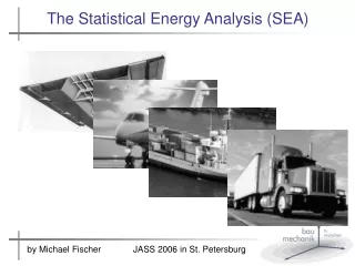
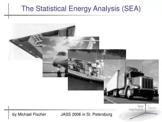
The Statistical Energy Analysis (SEA) S E A by Michael Fischer JASS 2006 in St. Petersburg
The Statistical Energy Analysis (SEA) • Methods used for vibration problems: by Michael Fischer JASS 2006 in St. Petersburg
The Statistical Energy Analysis (SEA) • Methods used for vibration problems: -Usually we are dealing with models like FEM, (BEM) and analytical models which enable us to calculate for deterministic loads and defined model parameters deterministic responses. -Typically the calculated value is given in detail with respect to frequency, time and location. -However, the level of discretization of time/frequency and the geometric data has to be defined at the basis of theoretical considerations regarding wave-lengths, eigenmodes etc. -The following introductory example shows, that at higher frequencies the reliability of the result of calculation might be considerably reduced. by Michael Fischer JASS 2006 in St. Petersburg
The Statistical Energy Analysis (SEA) 2. Introductory example: • room (25 m3) • limited by a steel plate • one of the boundary surfaces is excited by a harmonic load • 18 points in the room are considered by Michael Fischer JASS 2006 in St. Petersburg
The Statistical Energy Analysis (SEA) 2. Introductory example: • The figure shows for the 18 points • in the room all measured transfer • functions between the harmonic • load and the sound pressure. • lt can clearly be seen, that at • higher frequencies the transfer • functions differ considerably. Level difference sound pressure - harmonic force frequency Hz Hz Wheel of a bike by Michael Fischer JASS 2006 in St. Petersburg
The Statistical Energy Analysis (SEA) 2. Introductory example: - reason for the high differences: different contributions of single modes which are close together regarding their eigenfrequency. So e.g. in the centre of the room and a tonal excitation at 250 Hz, a difference of about 20 dB (factor 10) between the individual functions is observed. Level difference sound pressure - harmonic force frequency Hz Hz by Michael Fischer JASS 2006 in St. Petersburg
The Statistical Energy Analysis (SEA) 2. Introductory example: - Even slight temperatur differences in the room, which practically cannot be eliminated, influence the positions of the Eigenfrequencies so that a detailed prediction cannot be given Level difference sound pressure - harmonic force frequency Hz Hz by Michael Fischer JASS 2006 in St. Petersburg
The Statistical Energy Analysis (SEA) 2. Introductory example: • The air inside the room also shows • modes (starting at about 50 Hz) by Michael Fischer JASS 2006 in St. Petersburg
The Statistical Energy Analysis (SEA) 2. Introductory example: • Possible Uncertainties of… • boundary conditions (e.g. clamped/free edge) • dynamic material properties (e.g. concrete: E ~ 30kN/mm^2) • masses of the materials (e.g. concrete: 25 kN/m^2) • damping • load distribution (e.g. position of the machine) • frequency of excitation (e.g. velocity of train) • ... by Michael Fischer JASS 2006 in St. Petersburg
The Statistical Energy Analysis (SEA) 3. Historical example: In the early 1960s: -prediction of the vibrational response to rocket noise of satellite launch vecicles and their payloads -problem: the frequency range of significant response contained the natural frequencies of a multitude of higher order modes: -the Saturn launch vehicle possessed about 500.000 natural frequencies in the range 0 to 2000 Hz by Michael Fischer JASS 2006 in St. Petersburg
The Statistical Energy Analysis (SEA) 4. Motivation for SEA: • The both examples above are leading to the insight that • at higher frequencies a method with less detailing has to be accepted. • -A detailed analysis at the basis of FEM approach (input at a point of • excitation, output at a point of observation) would lead to results which • are very sensitive to slight changes in the input parameters • (factor 10!). • -In order to obtain acceptable sensitivities of the results, but to describe • nevertheless the system response, we will give the results in an averaged • sense. by Michael Fischer JASS 2006 in St. Petersburg
The Statistical Energy Analysis (SEA) 4. Motivation for SEA: by Michael Fischer JASS 2006 in St. Petersburg
The Statistical Energy Analysis (SEA) 5. Deterministic approach: modal superposition mode shape (point of observation) system response contribution of the i.th mode by Michael Fischer JASS 2006 in St. Petersburg
The Statistical Energy Analysis (SEA) 5. Deterministic approach: modal superposition influence of the geometry of excitation amplification functioninfluence of the frequency of excitation by Michael Fischer JASS 2006 in St. Petersburg
The Statistical Energy Analysis (SEA) 6. Energetic approach: 6.1 Shift to energy • In the first step a shift from velocities to energy is carried out. • the mean kinetic energy is proportional to the mean square velocity mode shape (point of observation) contribution of the i.th mode by Michael Fischer JASS 2006 in St. Petersburg
The Statistical Energy Analysis (SEA) 6. Energetic approach: 6.2 Averaging in the SEA • Now we increase the prediction accuracy by appropriate averaging • in several steps by Michael Fischer JASS 2006 in St. Petersburg
The Statistical Energy Analysis (SEA) 6. Energetic approach: 6.3 Averaging over the points of observation („ Step 1“) • by this step the phase information gets lost by Michael Fischer JASS 2006 in St. Petersburg
The Statistical Energy Analysis (SEA) 6. Energetic approach: 6.3 Averaging over the points of observation („ Step 1“) Orthogonality of modeshapes („Summing up the modal energy“) by Michael Fischer JASS 2006 in St. Petersburg
The Statistical Energy Analysis (SEA) 6. Energetic approach: 6.4 Averaging over the points of excitation („ Step 2“) • By this averaging, the information about the shape of the individual • eigenmodes is eliminated and has no longer to be considered • This means: the modes don‘t have to be calculated! by Michael Fischer JASS 2006 in St. Petersburg
The Statistical Energy Analysis (SEA) 6. Energetic approach: 6.4 Averaging over the points of excitation („ Step 2“) mean modal force modal mass by Michael Fischer JASS 2006 in St. Petersburg
The Statistical Energy Analysis (SEA) 6. Energetic approach: 6.4 Averaging over the points of excitation („ Step 2“) force amplification function total mass no information about the modes necessary! by Michael Fischer JASS 2006 in St. Petersburg
The Statistical Energy Analysis (SEA) 6. Energetic approach: 6.5 Averaging over the frequencies of excitation („ Step 3“) -To simplify the mean square velocity once again, we assume several similar modes N in a frequency band amplification by Michael Fischer JASS 2006 in St. Petersburg
The Statistical Energy Analysis (SEA) 6. Energetic approach: 6.5 Averaging over the frequencies of excitation („ Step 3“) force total mass damping frequency band by Michael Fischer JASS 2006 in St. Petersburg
The Statistical Energy Analysis (SEA) 6. Energetic approach: 6.5 Averaging over the frequencies of excitation („ Step 3“) Energy within a certain frequency band: centre frequency force frequency band total mass damping by Michael Fischer JASS 2006 in St. Petersburg
The Statistical Energy Analysis (SEA) 6. Mean input power -We are looking at one „sub-system“ (frequency band) -We assume a steady state vibration: „the mean input power, which is introduced during one cycle of vibration equals to the dissipated power due to damping“ (compare SDOF system). -mean input power in a frequency band: force frequency band total mass input power is independent from damping by Michael Fischer JASS 2006 in St. Petersburg
The Statistical Energy Analysis (SEA) 7. Balance of power- hydrodynamic analogy Mean input power P Energy E in the sub-system Dissipated energy by Michael Fischer JASS 2006 in St. Petersburg
The Statistical Energy Analysis (SEA) 7. Balance of power- hydrodynamic analogy -every sub-system is considered as a energy reservoir -The dissipated energy is proportional to the absolute dynamic energy E of the sub-system: damping by Michael Fischer JASS 2006 in St. Petersburg
The Statistical Energy Analysis (SEA) 7. Balance of power- hydrodynamic analogy Expansion to coupled systems: -For every sub-system holds: by Michael Fischer JASS 2006 in St. Petersburg
The Statistical Energy Analysis (SEA) 7. Balance of power- hydrodynamic analogy Expansion to coupled systems: -Energy flow between two sub-systems: modal energy coupling loss factor by Michael Fischer JASS 2006 in St. Petersburg
The Statistical Energy Analysis (SEA) 8. Equations of the SEA The governing equations can be derived by considering: the loss of energy by damping the energy flow between every pair of sub-systems (coupling) by Michael Fischer JASS 2006 in St. Petersburg
damping The Statistical Energy Analysis (SEA) 8. Equations of the SEA coupling by Michael Fischer JASS 2006 in St. Petersburg
The Statistical Energy Analysis (SEA) 8. Equations of the SEA -Related to the different possible deflection patterns (e.g. bending, shear, torsional waves): each part of the structure might appear as various energy reservoirs and thus described by various governing equations. -FE: usually a high dicretization of the structure is necessary -SEA: based on calculation of global values computational costs are much smaller interactive planning by the engineer is possible by Michael Fischer JASS 2006 in St. Petersburg
The Statistical Energy Analysis (SEA) 8. Conclusions and look into the future -Energy methods have a huge impact on the methodology of noise and vibration prediction -especially hybrid methods can carry out vibroacoustic investigations with a good confidence by Michael Fischer JASS 2006 in St. Petersburg
The Statistical Energy Analysis (SEA) 8. Conclusions and look into the future -example: by Michael Fischer JASS 2006 in St. Petersburg
Rail-Impedance-Model RIM The Statistical Energy Analysis (SEA) 8. Conclusions and look into the future by Michael Fischer JASS 2006 in St. Petersburg
The Statistical Energy Analysis (SEA) Thank you for your attention! by Michael Fischer JASS 2006 in St. Petersburg