Download
1 / 12
120 likes | 125 Views
8. Back-testing of trading strategies. 8.1Bootstrap Brock et al (1992), Davidson & Hinkley (1997), Fusai & Roncoroni (2008).

E N D
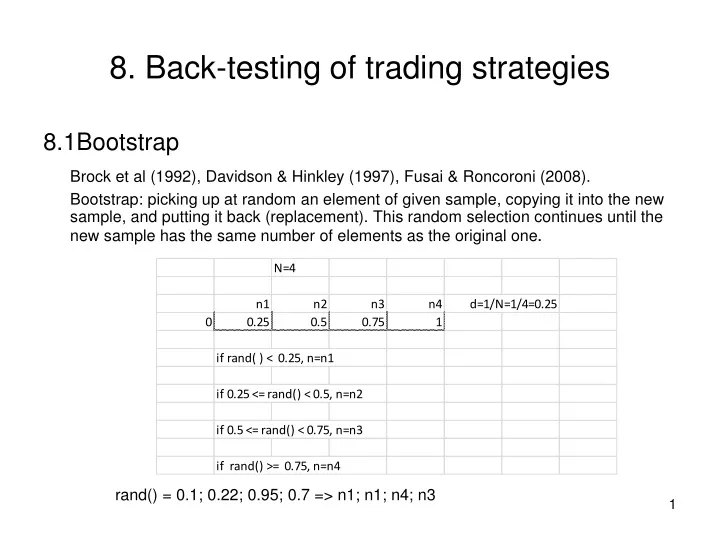
8. Back-testing of trading strategies 8.1Bootstrap Brock et al (1992), Davidson & Hinkley (1997), Fusai & Roncoroni (2008). Bootstrap: picking up at random an element of given sample, copying it into the new sample, and putting it back (replacement). This random selection continues until the new sample has the same number of elements as the original one. rand() = 0.1; 0.22; 0.95; 0.7 => n1; n1; n4; n3
8. Back-testing of trading strategies 8.1Bootstrap (continued) Block bootstrap (preserving autocorrelations) Replacement of L sequential data Stationary bootstrap for stationary (or weakly) samples: Block size L is drawn from the discrete geometric distribution Pr(L=k) = (1 – p)k-1p E[L] = 1/p => estimate of p
8. Back-testing of trading strategies 8.1Bootstrap (continued 2) 1. Model choice: random walk (with drift), ARMA, etc. 2. Bootstrapping residuals Example: AR(1) with log returns rt = log(Pt) - log(Pt-1) a) Estimate (with OLS) α and β for rt = α + βrt-1 + εt, εt = IID(0,σ2); σ2 = Var(εt) b) Calculate residuals et = rt - α - βrt-1 c) Generate new sample with bootstrapped residuals řt = α + βrt-1 + ět, d) Compile new price sample = exp(řt); = log(P1)
8. Back-testing of trading strategies 8.2 Markov chain Monte Carlo (MCMC) Markov process: generic stochastic process determined with relationships between their future, present, and past values. Future value for the Markov process of the 1st order is determined by its present value. Future value for the Markov process of the 2nd order is determined by its present value and the most recent past value, etc. The Markov processes of the 1st order cover a very wide class of dynamic short-memory phenomena including diffusional transfer (Brownian motion). Discrete Markov process => Markov chain. kth order: Pr(Xn = x | Xn-1 = xn-1, Xn-2 = xn-2,..., X1 = x1) = Pr(Xn = x | Xn-1 = xn-1, Xn-2 = xn-2,..., Xn-k = xn-k) Initial conditions: xn-1, ..., xn-k Stationarity: Pr(...) does not depend on n.
8. Back-testing of trading strategies 8.2 MCMC (continued) 1st order: Pr(Xn = x | Xn-1 = xn-1, ..., X1 = x1) = Pr(Xn = x | Xn-1 = xn-1) N2 probabilities pik = Pr(Xn = xi | Xn-1 = xk); i, k = 1, 2, ..., N => transition matrix. 2nd order: N3 probabilities pijk = Pr(Xn = xk | Xn-1 = xi, Xn-2 = xj) = pijk, i, j, k = 1, 2, ..., N
8. Back-testing of trading strategies 8.2 MCMC (continued 2) Implementation: Drawings from the uniform distribution are mapped onto transition probabilities for generating new samples. Long memory => higher order => computational challenges
MCMC Example Possible returns {-1, 0, 1} rk = -1: Pr(rk+1 =-1 | rk = -1) + Pr(rk+1 = 0 | rk = -1) + Pr(rk+1 = 1 | rk = -1) = 1 0.5 0.3 0.2 rk = 0: Pr(rk+1 =-1 | rk = 0) + Pr(rk+1 = 0 | rk = 0) + Pr(rk+1 = 1 | rk = 0) = 1 0.3 0.4 0.3 rk = 1: Pr(rk+1 =-1 | rk = 1) + Pr(rk+1 = 0 | rk = 1) + Pr(rk+1 = 1 | rk = 1) = 1 0.2 0.3 0.5 r1 = 0; rand() = 0.5, 0.2, 0.9, 0.1… => rk = 0, 0, -1, 1, -1,…
8. Back-testing of trading strategies 8.3 Random entry protocol What to do about coupled samples (e.g. price & some liquidity measure like aggregated volume at best price)? Do we want to destroy correlations between coupled samples? Autocorrelation bias... Implementation: Start trading at random point of time. Similar to block bootstrap but the block size is determined by timing of round-trip trading. But: limited number of entries...
8. Back-testing of trading strategies 8.4 Comparing trading strategies Data snooping in comparative testing on the same data sample... One problem: many strategies that were unsuccessful in the past are eliminated, so that only a small set of strategies is considered in the end, and the best of them is assumed to be the best among all. A newsletter scammer... Bootstrap reality check (BRC) (White (2000)) BRC is based on Lx1 (k=1, 2, …, L) statistic where L is the number of trading strategies, n is the number of prediction periods indexed from R to T, T = R + n + 1, is a vector of parameters that determine the trading strategies.
8. Back-testing of trading strategies 8.4 Comparing trading strategies (continued) Performance defined in terms of the excess return in respect to some benchmark determined with β0 (e.g. risk-free interest rate) fk,t+1(β) = ln[1 + yt+1Sk(ςt, βk)] – ln[1 + yt+1S0(ςt, β0)], k = 1, …, L yt+1 = (Xt+1 – Xt)/Xt, Xtis the original price series, Sk(ςt, βk) and S0(ςt, β0) are the trading signal functions that translate the price sequence ςt = {Xt-R, Xt-R+1, …, XT} into the market positions. The trading signal functions can assume values of 0 (cash), 1 (long position), and -1 (short position). Average return of strategy k: = E( fk)
8. Back-testing of trading strategies 8.4 Comparing trading strategies (continued 2) Null hypothesis: H0: max { } ≤ 0, k=1, ..., L; is average return of strategy k in respect to some benchmark (e.g. risk-free return) BRC: 1) Calculate = max { }, k = 1, ..., L 2) Perform stationary bootstrap for resamplingfk,i , i = 1, 2, ..., B (B is number of bootstrapped samples) and calculate their averages 3) Calculate = max {( - )}, i = 1, …, B k = 1, ..., L 4) Compare percentile of to : if it is higher than 1-p for given significance level p, the null hypothesis is rejected.
8. Back-testing of trading strategies 8.4 Comparing trading strategies (continued 3) Sullivan et al (1999): BRC on 100 years (1897 – 1996) of daily data for the Dow Jones. The strategy that is the best for given sample outperforms holding cash. However, the best in-sample strategy is not superior to the benchmark when tested out of sample. Hansen (2005): BRC may have a lower power due to possible presence of poorly performing strategies in the test. Power of the statistical test relates to the ability of rejecting false null hypothesis. Only promising strategies should be included in the test. Also, Romano & Wolf (2005), and Hsu et al (2009).