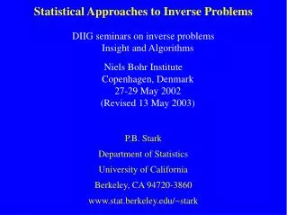
Statistical Measures of Uncertainty in Inverse Problems

Statistical Measures of Uncertainty in Inverse Problems Workshop on Uncertainty in Inverse Problems Institute for Mathematics and Its Applications Minneapolis, MN 19-26 April 2002 P.B. Stark Department of Statistics University of California Berkeley, CA 94720-3860 www.stat.berkeley.edu/~stark

Abstract Inverse problems can be viewed as special cases of statistical estimation problems. From that perspective, one can study inverse problems using standard statistical measures of uncertainty, such as bias, variance, mean squared error and other measures of risk, confidence sets, and so on. It is useful to distinguish between the intrinsic uncertainty of an inverse problem and the uncertainty of applying any particular technique for “solving” the inverse problem. The intrinsic uncertainty depends crucially on the prior constraints on the unknown (including prior probability distributions in the case of Bayesian analyses), on the forward operator, on the statistics of the observational errors, and on the nature of the properties of the unknown one wishes to estimate. I will try to convey some geometrical intuition for uncertainty, and the relationship between the intrinsic uncertainty of linear inverse problems and the uncertainty of some common techniques applied to them.

References & Acknowledgements Donoho, D.L., 1994. Statistical Estimation and Optimal Recovery, Ann. Stat., 22, 238-270. Evans, S.N. and Stark, P.B., 2002. Inverse Problems as Statistics, Inverse Problems, 18, R1-R43 (in press). Stark, P.B., 1992. Inference in infinite-dimensional inverse problems: Discretization and duality, J. Geophys. Res., 97, 14,055-14,082. Created using TexPoint by G. Necula, http://raw.cs.berkeley.edu/texpoint

Outline • Inverse Problems as Statistics • Ingredients; Models • Forward and Inverse Problems—applied perspective • Statistical point of view • Some connections • Notation; linear problems; illustration • Identifiability and uniqueness • Sketch of identifiablity and extremal modeling • Backus-Gilbert theory • Decision Theory • Decision rules and estimators • Comparing decision rules: Loss and Risk • Strategies; Bayes/Minimax duality • Mean distance error and bias • Illustration: Regularization • Illustration: Minimax estimation of linear functionals • Distinguishing Models: metrics and consistency

Inverse Problems as Statistics • Measurable space X of possible data. • Set  of possible descriptions of the world—models. • Family P = {Pq : q2Q} of probability distributions on X, indexed by models . • Forward operatorqaPq maps model  into a probability measure on X. Data X are a sample from Pq. Pq is whole story: stochastic variability in the “truth,” contamination by measurement error, systematic error, censoring, etc.

Models • Set  usually has special structure. •  could be a convex subset of a separable Banach space T. (geomag, seismo, grav, MT, …) • Physical significance of  generally gives qaPq reasonable analytic properties, e.g., continuity.

Forward Problems in Geophysics Composition of steps: • transform idealized description of Earth into perfect, noise-free, infinite-dimensional data (“approximate physics”) • censor perfect data to retain only a finite list of numbers, because can only measure, record, and compute with such lists • possibly corrupt the list with measurement error. Equivalent to single-step procedure with corruption on par with physics, and mapping incorporating the censoring.

Inverse Problems Observe data X drawn from distribution Pθ for some unknown . (Assume  contains at least two points; otherwise, data superfluous.) Use data X and the knowledge that  to learn about ; for example, to estimate a parameter g() (the value g(θ) at θ of a continuous G-valued function g defined on ).

Geophysical Inverse Problems • Inverse problems in geophysics often “solved” using applied math methods for Ill-posed problems (e.g., Tichonov regularization, analytic inversions) • Those methods are designed to answer different questions; can behave poorly with data (e.g., bad bias & variance) • Inference  construction: statistical viewpoint more appropriate for interpreting geophysical data.

Elements of the Statistical View Distinguish between characteristics of the problem, and characteristics of methods used to draw inferences. One fundamental property of a parameter: g is identifiable if for all η, z Θ, {g(η)  g(z)}  {PhPz}. In most inverse problems, g(θ) = θ not identifiable, and few linear functionals of θ are identifiable.

Deterministic and Statistical Perspectives: Connections Identifiability—distinct parameter values yield distinct probability distributions for the observables—similar to uniqueness—forward operator maps at most one model into the observed data. Consistency—parameter can be estimated with arbitrary accuracy as the number of data grows—related to stability of a recovery algorithm—small changes in the data produce small changes in the recovered model.  quantitative connections too.

More Notation Let T be a separable Banach space, T* its normed dual. Write the pairing between T and T* <•, •>: T*xTR.

Linear Forward Problems A forward problem is linear if • Θ is a subset of a separable Banach space T • X= Rn • For some fixed sequence (κj)j=1n of elements of T*, is a vector of stochastic errors whose distribution does not depend on θ.

Linear Forward Problems, contd. • Linear functionals {κj} are the “representers” • Distribution Pθ is the probability distribution of X. Typically, dim(Θ) = ; at least, n < dim(Θ), so estimating θ is an underdetermined problem. Define K : TRn Θ(<κj, θ>)j=1n . Abbreviate forward problem by X = Kθ + ε, θΘ.

Linear Inverse Problems Use X = Kθ + ε, and the knowledge θΘ to estimate or draw inferences about g(θ). Probability distribution of X depends on θ only through Kθ, so if there are two points θ1, θ2Θ such that Kθ1 = Kθ2 but g(θ1)g(θ2), then g(θ) is not identifiable.

Ex: Sampling w/ systematic and random error • Observe • Xj = f(tj) + rj + ej, j = 1, 2, …, n, • f 2C, a set of smooth of functions on [0, 1] • tj2 [0, 1] • |rj| 1, j=1, 2, … , n • jiid N(0, 1) • Take Q = C£ [-1, 1]n, X = Rn, and q = (f, r1, …, rn). • Then Pq has density • (2p)-n/2 exp{-åj=1n (xj – f(tj)-rj)2}.

Sketch: Identifiability Pz = Ph Pq  X = Rn K K X = K    g() g(h) g(z) R {Pz = Ph} ; {h = z}, so q not identifiable g cannot be estimated with bounded bias {Pz = Ph} ; {g(h) = g(z)}, so g not identifiable

Backus-Gilbert Theory Let Q = T be a Hilbert space. Let g 2T = T* be a linear parameter. Let {kj}j=1nµT*. Then: g(q) is identifiable iff g = L¢ K for some 1 £ n matrix L. If also E[e] = 0, then L¢ X is unbiased for g. If also e has covariance matrix S = E[eeT], then the MSE of L¢ X is L¢S¢LT.

Sketch: Backus-Gilbert Pq  X = Rn K X = K  L¢ X R g() = L¢ Kq

Backus-Gilbert++: Necessary conditions Let g be an identifiable real-valued parameter. Suppose θ0Θ, a symmetric convex set Ť T, cR, and ğ: ŤR such that: • θ0 + ŤΘ • For t Ť, g(θ0 + t) = c + ğ(t), and ğ(-t) = -ğ(t) • ğ(a1t1 + a2t2) = a1ğ(t1) + a2ğ(t2), t1, t2 Ť, a1, a2 0, a1+a2 = 1, and • supt Ť | ğ(t)| <. Then  1×n matrix Λ s.t. the restriction of ğ to Ť is the restriction of Λ.K to Ť.

Backus-Gilbert++: Sufficient Conditions Suppose g = (gi)i=1m is an Rm-valued parameter that can be written as the restriction to Θ of Λ.K for some m×n matrix Λ. Then • g is identifiable. • If E[ε] = 0, Λ.X is an unbiased estimator of g. • If, in addition, ε has covariance matrix Σ = E[εεT], the covariance matrix of Λ.X is Λ.Σ.ΛT whatever be Pθ.

Decision Rules A (randomized) decision rule δ: X M1(A) x δx(.), is a measurable mapping from the space X of possible data to the collection M1(A) of probability distributions on a separable metric space A of actions. Anon-randomized decision rule is a randomized decision rule that, to each x X, assigns a unit point mass at some value a = a(x)  A.

Estimators An estimator of a parameter g(θ) is a decision rule for which the space A of possible actions is the space G of possible parameter values. ĝ=ĝ(X) is common notation for an estimator of g(θ). Usually write non-randomized estimator as a G-valued function of x instead of a M1(G)-valued function.

Comparing Decision Rules • Infinitely many decision rules and estimators. Which one to use? The best one! But what does best mean?

Loss and Risk • 2-player game: Nature v. Statistician. • Nature picks θ from Θ. θ is secret, but statistician knows Θ. • Statistician picks δ from a set D of rules. δ is secret. • Generate data X from Pθ, apply δ. • Statistician pays lossl (θ, δ(X)). l should be dictated by scientific context, but… • Riskis expected loss: r(θ, δ) = Eql (θ, δ(X)) • Good rule d has small risk, but what does small mean?

Strategy Rare that one d has smallest risk 8qQ. • d is admissible if not dominated. • Minimaxdecision minimizes supqQr (θ, δ) over dD • Bayes decisionminimizes over dD for a given priorprobability distributionp on Q.

Minimax is Bayes for least favorable prior If minimax risk >> Bayes risk, prior π controls the apparent uncertainty of the Bayes estimate. Pretty generally for convex , D, concave-convexlike r,

Common Risk: Mean Distance Error (MDE) Let dG denote the metric on G. MDE at θ of estimatorĝof g is MDEθ(ĝ, g) = Eq [d(ĝ, g(θ))]. When metric derives from norm, MDE is called mean norm error (MNE). When the norm is Hilbertian, (MNE)2 is called mean squared error (MSE).

Bias When G is a Banach space, can define bias atθofĝ: biasθ(ĝ, g) = Eq [ĝ - g(θ)] (when the expectation is well-defined). • If biasθ(ĝ, g) = 0, say ĝis unbiased atθ (for g). • If ĝ is unbiased at θ for g for every θ, say ĝ is unbiased for g. If such ĝ exists, g is unbiasedly estimable. • If g is unbiasedly estimable then g is identifiable.

Sketch: Regularization  X = Rn K X = K  K error 0  g() g() bias R

Minimax Estimation of Linear parameters: Hilbert Space, Gaussian error • Observe X = Kq + e 2Rn, withq2QµT, T a separable Hilbert spaceQ convex{ei}i=1niid N(0,s2). • Seek to learn about g(q): Q!R, linear, bounded on Q For variety of risks (MSE, MAD, length of fixed-length confidence interval), minimax risk is controlled by modulus of continuity of g, calibrated to the noise level. (Donoho, 1994.)

Modulus of Continuity K  X = Rn   K  g(h) g(z) R

Distinguishing two models Data tell the difference between two models z and h if the L1 distance between Pz and Ph is large:

L1 and Hellinger distances

Consistency in Linear Inverse Problems • Xi = i + i, i=1, 2, 3, …  subset of separable Banach{i} * linear, bounded on  {i} iid  •  consistently estimable w.r.t. weak topology iff {Tk}, Tk Borel function of X1, . . . , Xk, s.t. , >0,  *, limkPq{|Tk - |>} = 0

Importance of the Error Distribution • µ a prob. measure on ; µa(B) = µ(B-a), a  • Pseudo-metric on **: • If restriction to  converges to metric compatible with weak topology, can estimate  consistently in weak topology. • For given sequence of functionals {ki}, µ rougher  consistent estimation easier.

Summary • Statistical viewpoint is useful abstraction. Physics in mapping   PPrior information in constraint . • Separating “model” from parameters of interest is useful: Sabatier’s “well posed questions.” • “Solving” inverse problem means different things to different audiences. Thinking about measures of performance is useful. • Difficulty of problem  performance of specific method.

Statistical Measures of Uncertainty in Inverse Problems