Download

1 / 29
290 likes | 438 Views
Static Optimization of Conjunctive Queries with Sliding Windows over Infinite Streams. Ahmed M.Ayad and Jeffrey F.Naughton Database Group University of Wisconsin. Presented by: Andy Mason and Sheng Zhong. Material is partially referenced from SIGMOD 2004 [1]. Overview. Introduction

E N D
Static Optimization of Conjunctive Queries with Sliding Windows over Infinite Streams Ahmed M.Ayad and Jeffrey F.Naughton Database Group University of Wisconsin Presented by: Andy Mason and Sheng Zhong Material is partially referenced from SIGMOD 2004 [1]
Overview • Introduction • Semantics of Sliding Window Continuous Queries • Cost Model • Load Shedding • Optimization Framework • Experiments
Introduction • The intent of the paper • Find a execution plan that minimizes resource usage when resources are sufficient • Find an execution plan that sheds tuples when resources are insufficient. • Given a continuous query in a steady state, each execution plan is similar to a Queuing Network System • Arriving tuples are clients • Query operators are servers • Execution plan is feasible if the system is stable • If the plan is infeasible, load shedding is needed
Feasible and Infeasible Query Plan 0.5+0.25<1 1+0.25>1 Load Shedding
Assumptions • The time stamps are unique (no ties) • Tuples arrive in the stream in a monotonically increasing order by its time stamp (no out of order arrival) • There is no relational tables involved in the query Discussion: Why will make these assumptions? Static optimization –> Rates of input streams are slow changing Enough memory to hold the buffering requirements for any query plan
Semantics • Definitions • Data Stream • Time-based Window • Tuple-based Window • Selection • A filter takes a stream as input and outputs a stream • Join • A symmetric operator that takes two input streams The cost model
Rate and Window Calculations • 1 Select output rate • 2 Active window size • 3 output rate of window join • 4 Active size of window join • 5 output rate of n-ary join of n streams • 6 Active window size of n-ary join
Cost Model SELECT A.a, B.b, C.c FFROM A [ROWS 10] B [ROWS 10] C [ROWS 10] WHERE A.a = B.a AND B.b = C.b • An concrete example on the application of the cost model
Load Shedding • A form of approximation which reduces load by dropping tuples from the incoming streams • Methods of Load Shedding • Random dropping of tuples Presented in this paper • Achieved by inserting random drop boxes at several points in the query plan • Semantic dropping of tuples • Goal – Maximize output rate of the approximated query • Problems addressed: • Optimal placement of drop boxes in an execution plan and the optimal setting of their sampling rate • Choice of plan to shed load from
Selection Only Queries • Initial condition • A query consisting of n consecutive filters • An execution plan for it that orders the filters in asc order by a designated number • n+1 possible combinations • Observation: Only need to drop tuples directly from the streaming source before they are processed by any of the filters • Conclusion: The plan with the lowest cost yields the highest rate
Join Queries • Only consider tuple-based windows • Shedding Load From a Specific Plan • Choice of Plan for Load Shedding
Shedding Load from a Specific Plan • Where do we put the drop boxes? • Query plan joining n streams • Binary joins • Drop box can be put before each of the two inputs to the n - 1 join operators • Plus a box right after the last join is performed • 2n - 1 possible locations Obs: Sufficient to drop tuples from the input sources before they are processed by any join operator
Choice of Load Shedding Plan • Intuition for Selection queries • Pick plan with lowest resource utilization • Join queries • Plan with lowest resource utilization? • This intuition does not always work • Why?
Load Shedding Plan Example • Plans shed load in the order of their average utilization • Switch-over occurs ~ 4.5 milliseconds (plan b=best)
Observations from Example • The plan with the lowest utilization is not always the best choice for shedding load • When the join cost is ~ 14 milliseconds, the throughput of the best plan is more than twice the throughput of the lowest utilization plan • Lowest utilization plan could be the worst choice • Conclusion: Load shedding must be integrated in the optimization process
Optimization Framework • Two areas • Throughput of the plan • Utilization cost of the plan • Feasible queries • Goal: Minimize cost of the plan • Where throughput is fixed at its maximum value for all feasible queries • Infeasible queries • Goal: Maximize throughput of the plan • Where cost is fixed at its maximum value for all p • Assumption • Search space of alternative plans always equipped with drop boxes • All plans in the search space will be feasible • Problem can be treated as unconstrained
Optimization Goal • Maximize • R(p) = plan throughput/plan cost • Simplest optimization algorithm • Generate the set of all plans of the query • For each plan in the set • Compute cost of the plan • If cost > 1, insert drop boxes • Compute R • Return the plan that maximizes R(p)
Heuristic Optimizer • Based on the original System R optimizer • Builds the plan from the bottom-up by storing the best plans for successively larger subsets of the input streams • Computing the best plan for any subset • Test whether this subplan is feasible • If infeasible, tune the values of the drop boxes placed at its input streams using load shedding alg
Computing the best subset plan • Test whether this subplan is feasible • If infeasible, tune the values of the drop boxes placed at its input streams using load shedding alg • Store subplan • At any stage • If a drop box is placed in front of a stream which had another one from a previous round, the two are combined into one drop box whose selectivity is the product of the original two
Experiment Setup • 1000 random continuous queries • Each query reps join of five input streaming sources: A, B, C, D, E • Window sizes and join selectivities fixed • Rates were randomly picked from 10 to 1000 tuples/sec
Average Gain in Throughput over using the Lowest Utilization Plan At very low resources, the gain is very significant (almost 8 folds at the 1% mark)
Heuristic Optimizer Except at very low resources, the performance of the heuristic optimizer is quite impressive
Summary • Presented framework for static optimization of sliding window conjunctive queries over infinite streams • Cost Model • Load Shedding • Load shedding must be integrated in the optimization process! • Optimization Framework • Experimental Results
References [1] http://web.cs.wpi.edu/~cs525/f06s-EAR/cs525-homepage_files/LITERATURE/SIGMOD04-opt-shed-wisconsin.pdf [2] http://se.uwaterloo.ca/~tozsu/courses/cs856/F05/Presentations/Week8/Stream_Maryam.pdf