Download
1 / 41
410 likes | 715 Views
POPULATION DYNAMICS. READINGS: FREEMAN, 2005 Chapter 52 Pages 1196-1213. MATURNITY TABLE AND REPRODUCTIVE OUTPUT. Fecundity is the number of female offspring produced by each female in a population. A maternity table combines survivorship (l X ) with age specific fecundity (m X ) .

E N D
POPULATION DYNAMICS READINGS: FREEMAN, 2005 Chapter 52 Pages 1196-1213
MATURNITY TABLE AND REPRODUCTIVE OUTPUT • Fecundity is the number of female offspring produced by each female in a population. • A maternity table combines survivorship (lX) with age specific fecundity (mX) . • Net reproductive output, ∑ (lX mX), provides a way of projecting population changes each generation.
RO AND POPULATION DYNAMICS The following rules can be used to determine if a population is stationary, increasing or decreasing. The rules are: • If Ro = 1, then population is stationary. • If Ro > 1, then population is growing. • If Ro < 1, then population is declining.
DISTRIBUTION OF BIRTHS AND REPRODUCTIVE OUTPUT In populations that have similar age specific survivorship curves: • First births at early ages increase Ro . • First births at late ages decrease Ro . Delaying births in a growing population will slow the rate of growth.
CHANGING SURVIVORSHIP AS A MANAGEMENT TOOL • Age specific mortality and natality data can be used to make management decisions in harvesting or conserving wildlife populations. • Assume that a population of interest is growing at too high a rate, what are the consequences of harvesting old versus young individuals on changing the rate of population growth?
LIFE HISTORY CHARACTERISTICS • Population attributes such as lifespan, mortality and natality patterns, biotic potentials, and patterns of population dynamics are called life history characteristics. • Life history characteristics have important consequences for wild life management.
FOUR IMPORTANT ASPECTS OF LIFE HISTORIES • 1. Lifespan --- the upper age limit for the species. • 2. Mortality --- the pattern of survivorship (I, II, or III). • 3. Natality --- the age to reproductive maturity and number of offspring produced. • 4. Biotic potential --- maximum rate of natural increase (rmax = births - deaths).
Short-lived. Type III survivorship high juvenile mortality; relatively secure old age. Many offspring from young adults. High maximum rate of population growth. Long-lived. Type I survivorship: low juvenile mortality; high mortality at old age. Few offspring from older adults. Low maximum rate of population growth. LIFE HISTORY EXTREMES
LIFE HISTORY TRAITS FORM A CONTINUUM • Every species can be placed somewhere on a continuum with respect to the life history extremes. • Comparisons of life histories are best done between species that show similar evolutionary histories. • For example, comparisons of field mice (short-lived) with muskrats (long-lived); both are rodents in closely related taxonomic families. • See Freeman (2005) page 1195 for more.
DISCRETE VS CONTINUOUS POPULATION GROWTH • Discrete generations. Most species reproduce only once a year. The breeding season is most commonly in late winter or early spring. • Continuous or over-lapping generations. A few species are capable of breeding throughout the year.
DISCRETE POPULATION GROWTH • The simplest way to express population growth rate is to compare the number of individuals at the start of the breeding season to the number at the start of the following year’s breeding season. • A mathematical model is N1/No = ; where No original population size, N1 size one year later and is rate of change. Thus, N1 = No or Nt = Not
CONTINUOUS POPULATION GROWTH • The growth rate of such a population is in fact the population’s per capita growth rate; it is symbolized as r (the instantaneous rate of increase. • A mathematical model is = er ; where is rate of change and e is the base of the natural log (2.72). Thus, Nt = No ert . • In most cases r ≈ Ro /g ; where g is the generation time.
EXPONENTIAL GROWTH • Since Nt = No ert, a constant value for r will result in an accelerating change (∆) in N with passing time (t). • In this example, N doubles with every unit increase in t.
Developing and Applying Population Growth Equations • Freeman (2005) in Box 52.2 gives a detailed description of Discrete and Continuous growth models. See pages 1197- 1199. • Solve problems 1-4 on page 1199.
DOUBLING TIME • A useful way for projecting exponentially growing populations. • Simply the time that it takes for a population to double (x2). • Where Nt = No ert , the special case where Nt/No = 2 or ert = 2 or Nt = No *2.
A DOUBLING TIME PROBLEM • PROBLEM: If 20 individuals were alive at the start of t = 0 and the per capita rate of increase (r) is 2% per year, how many years will it take the population to double (Nt/No = 2 )? • SOLUTION: 40 = 20 e0.02t or ln(2) = 0.02 *t or 0.693117 = 0.02 *t or 0.693117/0.02 = t =34.6 or 35 years.
EXPONENTIAL GROWTH • Exponential growth occurs when births exceed deaths giving rise to a constant positive r. • When r is constant and positive, ∆N accelerates with every unit change in t.
EXPONENTIAL DECLINE • Exponential decline occurs when deaths exceed births giving rise to a constant negative r. • When r is constant and positive, ∆N decelerates with every unit change in t.
POPULATION FLUCTUATIONS • Population fluctuations occur when births and deaths are random variables such that r averages around 0. • When r fluctuates around 0, N remains more or less constant.
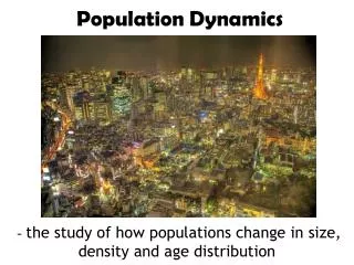
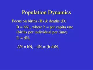
ABUNDANCE OF HOMO SAPIENS • Birth rates are expressed as number of births per 1,000 people per year. • Death rates are expressed as number of deaths per 1,000 people per year. • The instantaneous rate of increase r is often called rate of natural increase and equals births minus deaths or r = b - d.
Some Human Population Data dN/dt ~8 individuals every 2 seconds in 2005
Doubling Times Associated With Rates of Natural Increase ( r )
AGE STRUCTURES • The relative proportions of people at various ages reflect the age structure of a population. • High rates of natural increase result in ever-increasing numbers of young people (an age pyramid). • “Flat” age structures are indicators of stationary population sizes.
AGE STRUCTURE OF A RAPIDLY GROWING POPULATION • This age structure is found in rapidly growing populations. • The high proportion of younger relative to older age groups is a sign of rapid growth. • Note that over half of the population is 19 or under.
AGE STRUCTURE OF A SLOW GROWING POPULATION • This population is approaching zero growth (stasis). • A stationary population has age groups that are relatively uniform in size. • Where are you in this age structure?
AGE STRUCTURE OF A DECLINING POPULATION • This population has just passed zero growth and is entering a declining phase. • Note the high proportion of older relative to younger age groups.
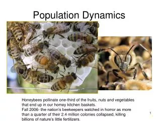
DYNAMICS OF ANIMAL POPULATIONS • Introductions of pheasant and turkey populations often result in exponential growth. • Population cycles such as seen in the red grouse have been experimentally examined as being caused by parasites and male aggression. • Threatened or endangered populations of lizards, fritillary butterflies, and Leadbeaters possum have been studied.
EXPONENTIAL GROWTH OF INTRODUCED POPULATIONS • 50 some pheasents were placed on an island in Pudget Sound the population increased to over 1,000 in only 5 years. • Male wild turkeys were reintroduced into Michigan in 1970 and increased exponentially into the 1990’s.
RED GROUSE POPULATION CYCLES • Freeman describes experiments designed to test the hypothesis that population cycles are due to density-dependent parasite infections. • Other experiments implicate density- dependent male aggression.
DECLINING ANIMAL POPULATIONS HAVE BEEN STUDIED • Freeman describes demographic studies of a European lizard species that is declining in some areas. • He explains how migration maintains some local populations in spite of local extinction. • He presents a model of how migration rates are likely to influence population viability of an endangered marsupial.
POPULATION DYNAMICS READINGS: FREEMAN, 2005 Chapter 52 Pages 1196-1213