Download
1 / 52
560 likes | 936 Views
Percolation and Polymer-based Nanocomposites. Avik P. Chatterjee Department of Chemistry State University of New York College of Environmental Science & Forestry. Outline. Fiber-based composites & percolation: the “What” and the “Why” Elastic moduli in rod-reinforced nanocomposites:

E N D
Percolation and Polymer-based Nanocomposites Avik P. Chatterjee Department of Chemistry State University of New York College of Environmental Science & Forestry
Outline • Fiber-based composites & percolation: the “What” and the “Why” • Elastic moduli in rod-reinforced nanocomposites: A unified model that integrates percolation ideas with effective medium theory • Analogy between continuum rod percolation and site percolation on a modified Bethe lattice: calculation of the percolation threshold and percolation and backbone probabilities • A simple model for systems with non-random spatial distributions for the fibers: Effects due to particle clustering and correlation • Future Directions and Acknowledgements
Composites & Percolation • Composites: Mixtures of particles/nanoparticles (the “filler”), dispersed (randomly or otherwise) within another phase (the “matrix”) • Basic idea: to combine & integrate desirable properties (e.g., low density, high mechanical moduli or conductivity) from different classes of material • Natural Composites (e.g. bone and wood) often exhibit hierarchical structures, varying organizational motifs on different scales • “Wood for the Trees” : wood remains one of the most successful fiber-reinforced composites, and cellulose the most widely-occurring biopolymer (annual global production of wood ~ 1.75 x 10⁹ metric tons)
Wood: A natural, fiber-reinforced composite Cell walls: layered cellulose microfibrils (linear chains of glucose residues, degree of polymerization 5000 – 10000, 40-50 % w/w of dry wood depending on species), bound to matrix of hemicellulose and lignin R.J. Moon, “Nanomaterials in the Forest Products Industry”, McGraw-Hill Yearbook in Science & Technology, p. 226 -229, 2008
Cellulose Nanocrystals (I) • Cellulose (linear chains of glucose residues), bound to matrix of lignin and hemicellulose, comprises 40-50 % w/w of dry wood • Individual fibers have major dimensions ~ 1-3 mm, consisting of spirally wound layers of microfibrils bound to lignin-hemicellulose matrix; microfibrils contain crystalline domains of parallel cellulose chains; individual crystalline domains ~ 5-20 nm in diameter, ~ 1-2 m in length • Nanocrystalline domains separable from amorphous regions by controlled acid hydrolysis (amorphous regions degrade more rapidly) • Crystalline domain elastic modulus (longitudinal) ~ 150 GPa: compare martensitic steel ~ 200 GPa, carbon nanotubes ~ 103 GPa • Suggests possible role for cellulose nanocrystals as a renewable, bio- based, low-density, reinforcing filler for polymer-based nanocomposites
Cellulose Nanocrystals (II) • Cellulose microfibrils secreted by certain non-photosynthetic bacteria (e.g. Acetobacter xylinum), and form the mantle of sea-squirts (“tunicates”) (e.g. Ciona intestinalis) • These highly pure forms are free from lignin/hemicelluloses; fermentation of glucose a possible microbial route to large-scale cellulose production. Nanocrystalline cellulose whiskers, from acid hydrolysis of bacterial cellulose. Image courtesy of Profs. W.T. Winter and M. Roman, Dept. of Chemistry, SUNY-ESF, and Dept. of Wood Science and Forest Products at Virginia Tech. Adult sea-squirts
Connectedness Percolation: What ? Percolation:The formation of infinite, spanning clusters of “connected” (defined by spatial proximity) particles. : Below percolation threshold : Above percolation threshold
Percolation: Why? Dramatic Effects on Material Properties Impact Toughness: Z. Bartczak, et al., Polymer, 40, 2331, (1999) Izod impact energy (J/m) Average ligament thickness (mm) t – Matrix ligament thickness Toughness of HDPE/Rubber Composites Rubber particle size range: 0.36 ~ 0.87 mm
Electrical conductivity and Elastic Modulus (I) • Polypyrrole-coated cellulose whiskers investigated as electrically conducting filler particles: (L. Flandin, et al., Compos. Sci. Technol., 61, 895, (2001); Mean aspect ratio 15) • Mechanical reinforcement/modulus enhancement: (tunicate cellulose whiskers in poly-(S-co-BuA), V. Favier et al., Macromolecules, 28, 6365, (1995); Mean aspect ratio 70)
Electrical conductivity and Elastic Modulus (II) • Polystyrene (PS) reinforced with Multi-Walled Carbon Nanotubes (MWCNTs): (Diameters: 150 – 200 nm; Lengths: 5 – 10 m; T = 190o C; critical volume fraction 0.019; A.K. Kota, et al., Macromolecules, 40, 7400, (2007))
Percolation Thresholds for Rod-like Particles Percolation threshold for rods, * (D / L), depends approximately inversely upon aspect ratio, a result supported by: (i) Integral equation approaches based upon the Connectedness Ornstein- Zernike equation (X. Wang, A.P. Chatterjee, J. Chem. Phys., 118, 10787, (2003); R.H.J. Otten and P. van der Schoot, Phys. Rev. Lett. 103, 225704, (2009)) (ii) Monte-Carlo simulations of both finite-diameter as well as interpenetrable rods(L. Berhan, A.M. Sastry, Phys. Rev. E, 75, 041120, (2007); M. Foygel, et al., Phys. Rev. B, 71, 104201, (2005)) (iii) Excluded volume arguments (I. Balberg, et al.,Phys. Rev. B 30, 3933-3943, (1984))
Elasticity: Stress, Strain, & Stiffness • Stress tensor: { } (Energy/Volume) • Strain tensor: { } (Dimensionless) • Stiffness tensor: {C} (Energy/Volume): Fourth rank tensor • {C} can have a maximum of 21 independent elements/elastic coefficients • For an isotropic system, there are only TWO independent elastic constants, usually chosen from amongst: {E, G, K, } (tensile, shear, and bulk modulus, and Poisson ratio, respectively) • In terms of deformation energy per unit volume, U : and: , where:
A Seismic Interlude • Seismic (earthquake-generated) waves: • Primary/Pressure (“P-waves”): Longitudinal 5-7 km/s in crust, 8 km/s in mantle • Secondary/Shear (“S-waves”): Transverse 3-4 km/s in crust, 5 km/s in mantle Cannot traverse liquid outer core of the earth • “Shadow zones” and travel times reveal information regarding internal structure of the earth (Courtesy US Geological Survey)
Elastic Moduli of Composite Materials • Simple estimates employing only: (i) the volume fractions {n}, and: (ii) the elastic coefficients {En}, of the individual constituents, include the Voigt- Reuss and Hashin-Shtrikman bounds (for isotropic materials) (Z. Hashin, S. Shtrikman, J. Mech. Phys. Solids, 11, 127, (1963)) • Arithmetic mean (“Hill average”) of such bounds frequently employed as a semi-empirical tool (R. Hill, Proc. Phys. Soc. London A, 65, 349, (1952); S. Ji, et al., J. Struct. Geol., 26, 1377, (2004)) Voigt / “Parallel” Reuss / “Series”
Percolation and Elastic Moduli • Cellulose nanocrystals modeled as circular cylinders, uniform radius R, variable lengths L • Nanocrystals modeled as being transverselyisotropic, with five independent elastic constants: {Eax, Etr, Gtr, ax, tr} • Eax = 130 GPa, Etr = 15 GPa, Gtr = 5 GPa, ax = tr = 0.3 (L. Chazeau, et al., J. Appl. Polym. Sci., 71, 1797, (1999)) • Actual unit cell symmetry: monoclinic, implying 13 independent elastic constants (K. Tashiro, M. Kobayashi, Polymer, 32, 1516, (1991)) • Objective: To unify percolation ideas with effective medium theory towards an integrated model for composite properties 2 R L
Model for Network Contribution to Elasticity • For network element of length L and radius R: elastic deformation energy U is: Combines stretching, bending, shearing energies, {ij } are strain components in fiber-fixed frame, with fiber axis in the Z-direction (F. Pampaloni, et al., Proc. Natl. Acad. Sci. US., 103, 10248, (2006)) • Assume: (i) isotropic orientational distribution, (ii) random contacts between rods, Poisson distribution for lengths of network elements, and (iii) affine deformation • Energy of elastic deformation averaged over rod and segment lengths and orientations, strain tensor transformed to laboratory frame, then differentiated twice with respect to {ij } to obtain estimates for the network moduli {Enet, Gnet} • BUT:Rods of different lengths will differ in likelihood of belonging to network, and for small enough volume fractions, no network exists !
Percolation Probability and Threshold • Percolation probability, denoted P (, L) = probability that a randomly selected rod of length L belongs to the percolating network/infinite cluster • Modeled as: for , and zero otherwise • , L-dependent percolation threshold • Parameters { } are treated as adjustable: control transition width & location of threshold • These assumptions, together with piecewise-linear (unimodal) model for the overall distribution over rod lengths L, allows estimation of: (i) volume fraction of rods belonging to network (net), (ii) volume fraction and length distribution of rods that remain dispersed, (iii) average length of network elements (assuming random contacts) • There remains the task of combining the network moduli with contributions from the matrix, and from the dispersed rods
Moduli for the Composite • Identify a “continuum surrogate” for network, using “Swiss cheese” analogy, where: (matrix + dispersed rods) (spherical voids) • Use Mori-Tanaka (MT) model to estimate moduli for an isotropic system made up of: (matrix + dispersed rods) (Dispersed rods treated as length-polydisperse, within a discrete two-component description) (Y.P. Qiu, G.J. Weng, Int. J. Eng. Sci.,28, 1121, (1990)) • Final step: again use Mori-Tanaka (MT) method to estimate moduli for the system: (continuum network surrogate) + (spherical voids now filled with isotropic system of {matrix + dispersed rods}, with moduli determined in previous step) • Recursive use of MT model: equivalent in this context to Hashin-Shtrikman upper bound
Results (I) • Matrix: Copolymer of ethylene oxide + epichlorohydrin (EO-EPI) • Filler: Tunicate cellulose whiskers (solution cast system) • Mean whisker radius R = 13.35 nm • Whisker Lengths: Ln = 2.23 m, Lmax = 5.37 m (reproduces first two moments of experimentally measured distribution) • Solid Line: Polydispersity in rod lengths included in model • Broken Line: Model treats rods as monodisperse, J.R. Capadona, et al., Nat. Nanotechnol., 2, 765, (2007); D.A. Prokhorova, A.P. Chatterjee, Biomacromolecules, 10, 3259, (2009)
Results (II) • Matrix: waterborne polyurethane (WPU) • Filler: Flax cellulose nanocrystals • Mean whisker radius R = 10.5 nm • Whisker Lengths: Ln = 327 nm, Lmax = 500 nm (based on experimentally measured distribution of rod lengths) • Solid Line: Polydispersity in rod lengths included in model • Broken Line: Model treats rods as monodisperse, X. Cao, et al., Biomacromolecules, 8, 899, (2007); D.A. Prokhorova, A.P. Chatterjee, Biomacromolecules, 10, 3259, (2009)
Results (III) • Matrix: Copolymer of styrene + butyl acrylate (poly-(S-co-BuA)) • Filler: Tunicate cellulose whiskers • Mean whisker radius R = 7.5 nm • Whisker Lengths: Ln = 1.17 m, Lmax = 3.0 m (based on experimentally measured distribution of rod lengths) • Solid Line: Polydispersity in rod lengths included in model • Broken Line: Model treats rods as monodisperse, M.A.S.A. Samir, F. Alloin, A. Dufresne, Biomacromolecules, 6, 612, (2005); D.A. Prokhorova, A.P. Chatterjee, Biomacromolecules, 10, 3259, (2009)
Can Continuum Rod Percolation be related to Percolation on the Bethe Lattice ? • Perfect dendrimer/Cayley tree, with uniform degree of branching = z at each vertex • No loops/closed paths available • Extensively studied as exemplar of mean-field lattice percolation (M.E. Fisher, J.W. Essam, J. Math. Phys., 2, 609, (1961); R.G. Larson, H.T. Davis, J. Phys. C, 15, 2327, (1982)) • If vertices are occupied with probability , then site percolation threshold located at: * = (1/(z – 1)) Portion of a Bethe lattice with z = 3 • Given how thoroughly this problem has been examined,question arises whether one can relate continuum rod percolation to percolation on the Bethe lattice
Continuum Rod Percolation Bethe Lattice:A simple-minded mapping: • Consider a population of rods, with uniform radius = R, but variable lengths L. We let denote the distribution over rod lengths • On average: a rod of length L experiences (L/R) contacts with other rods in the system • For a Bethe lattice with degree z: each occupied site has (on average) z “contacts” with nearest neighbor occupied sites • Suggests the following analogy: Rod Occupied lattice site z z (L) (L/R) The corresponding Bethe lattice must have a distribution of vertex degrees
Percolation on a modified Bethe Lattice • Bethe Lattice Analog: Site percolation on a modified Bethe lattice, with site occupation probability = , and with vertex degree distribution f (z) that can be obtained from the underlying rod length distribution • Let = Probability that a randomly chosen branch in such a lattice, for which it is known that one of the terminal sites is occupied, does not lead to the infinite cluster • Given the absence of closed loops, is determined by: (M.E.J. Newman, et al., Phys. Rev. E, 64, 026118, (2001); M.E.J. Newman, Phys. Rev. Lett., 103, 058701, (2009)): Illustration of a portion of modified Bethe lattice where the summation runs over all values of z (L), and depends only upon and f (z)
Percolation Threshold and Probability: • Percolation probability for a rod of length L = probability that an occupied site with vertex degree z (L) belongs to the infinite cluster • Percolation threshold = value of at which a solution exists for other than the trivial solution { = 1, P = 0}: for the case that L >> R for all rods in the system (A.P. Chatterjee, J. Chem. Phys., 132, 224905, (2010); an identical result was derived in the field of “scale free” (power law) networks some years ago, R. Albert, A.-L. Barabasi, Rev. Mod. Phys., 74, 47, (2002)) • Percolation threshold governed by weight-averaged aspect ratio: consistent with results from an integral equation-based study: (R.H.J. Otten, P. van der Schoot, Phys. Rev. Lett., 103, 225704, (2009))
Generalization to finite-diameter rods: • Model rods as hard core + soft shell entities: hard core radii and lengths denoted: {R, L}, and soft shell radii and lengths given by: {R + l, L + 2 l} • For this problem, an identical approach yields: (A.P. Chatterjee, J. Statistical Physics, 146, 244, (2012)): • This is in full agreement with recent findings based on integral equation approach, for arbitrarily correlated joint distributions over rod radii and lengths (R.H.J. Otten, P. van der Schoot, Phys. Rev. Lett.103, 225704, (2009), J. Chem. Phys. 134,094902, (2011)) • Result can be generalized to particles with arbitrary cross-sectional shapes, not just circular cylinders (A.P. Chatterjee, J. Chem. Phys., 137, 134903, (2012))
Network and Backbone Volume Fractions: • A particle is said to belong to the “backbone” of the network if it experiences at least two contacts with the infinite cluster • Let B (z (L)) = Probability that a rod of length L belongs to the backbone • Then: (R.G. Larson, H.T. Davis, J. Phys. C, 15, 2327, (1982)) • Volume fractions occupied by the network, and network backbone: • Near Threshold: where Lw , Lz are weight and z-averaged rod lengths, respectively (A.P. Chatterjee, J. Chem. Phys., 132, 224905, (2010))
Illustrative Results for Percolation & Backbone Probabilities: • Polydisperse Rods: Unimodal Beta distribution, with: Lmin= 8.33 R, Lmax= 800 R, Ln= 66.67 R, Lw= 100 R = 1.5 Ln, Lz= 133.34 R = 2 Ln : Black curves • Monodisperse Rods (for comparison): Ln= Lw= Lz= 100 R, same percolation threshold as the polydisperse rod population: Red curves Upper Black Curves: L = Lmax Lower Black Curves: L = Lmin
Network & Backbone Volume Fractions: • Polydisperse Rods: Unimodal Beta distribution, with: Lmin= 8.33 R, Lmax= 800 R, Ln= 66.67 R, Lw= 100 R = 1.5 Ln, Lz= 133.34 R = 2 Ln : Black curves • Monodisperse Rods (for comparison): Ln= Lw= Lz= 100 R, same percolation threshold as the polydisperse rod population: Red curves Network, backbone, volume fractions lower for polydisperse system
Comparison with Monte Carlo Simulations: • Monte Carlo (MC) simulations for various polydisperse rod systems (B. Nigro et al., Phys. Rev. Lett., 110, 015701, (2013)) • MC results show reasonable agreement with theory p = Number fraction of long rods for bidisperse systems Symbols = MC results, various values of p and distributions of aspect ratios Solid Line = Theory based upon modified Bethe lattice
Average number of Contacts at Threshold: • Average number of contacts per particle at threshold: where z is the vertex degree in the modified Bethe lattice • For polydisperse systems, Nc can be smaller than unity • MC results show qualitative agreement with this result (B. Nigro et al., Phys. Rev. Lett., 110, 015701, (2013)) p = Number fraction of long rods, bidisperse systems Symbols = MC results, various aspect ratio distributions A similar result (Nc < 1) has been reported for hyperspheres in high-dimensional spaces (N. Wagner, I. Balberg, and D. Klein, Phys. Rev. E 74, 011127, (2006))
Non-random Spatial Distribution of Particles: Clustering and Correlation Effects: • Foregoing results assume particles are distributed in a spatially random, homogeneous fashion • But: particle distribution may in reality display local clustering or aggregation, particle contact numbers may be altered by correlation effects: “Quality of dispersion” can be variable • VERY SIMPLE & STRICTLY OPERATIONAL microstructural descriptors that capture such mesoscale non-randomness: (i) Clustering parameter, p : Measures degree of clustering (ii) Correlation parameter, K : Measures degree of rod-rod correlation, using the Quasi-Chemical Approximation (“QCA”) • Model separates effects upon percolation due to (i) polydispersity, (ii) clustering, and (iii) particle correlation
Parameters quantifying degrees of Clustering and Correlation: • CLUSTERING:p = Number fraction of sites with a given vertex degree z that enjoy fully tree-like local environments; the remainder belong to fully connected subgraphs • p relates inversely to “Clustering coefficient”, C, where C = Probability that a pair of rods X and Y, each of which touches a given (other) rod Z, also touch each other (D.J. Watts and S.H. Strogatz, Nature, 393, 440, (1998)) • CORRELATION: , where: = probability that any randomly selected pair of directly connected sites have the occupancy states i and j • p = 1 Fully unclustered, and p = 0 Maximally clustered • Increase in K Fewer rod-rod contacts for fixed rod volume fraction, rods more likely to be entirely enveloped by matrix
Modified Bethe Lattice to address Particle Clustering Effects: • Modified lattice includes fraction of fully connected subgraphs to model particle clustering (p) • Correlation between occupation states of neighboring sites described within QCA (K) • Percolation threshold can be expressed as function of: (i) polydispersity, (ii) degree of clustering, and (iii) strength of rod-rod correlations. Volume fractions occupied by network and network backbone, and percolation probabilities, can also be estimated • Clustering raises the percolation threshold, and correlations that increase the number of rod-rod contacts lower the percolation threshold (M.E.J. Newman, Phys. Rev. Lett., 103, 058701, (2009); A.P. Chatterjee, J. Chem. Phys., 137, 134903, (2012))
Effects of Particle Clustering on Conductivity in Nanotube Networks: • Percolation theory + Critical Path Approximation (“CPA”) leads to • model for electrical conductivity (V. Ambegaokar, B.I. Halperin, and J.S. • Langer, Phys. Rev. B, 4, 2612, (1971); G. Ambrosetti, et al., Phys. Rev. B, 81, • 155434, (2010)) • For given (i) volume fraction, • (ii) polydispersity, and degrees • of (iii) clustering and • (iv) correlation, determine the • soft shell thickness for which • particles just form a percolating • cluster/network • = soft shell thickness, and: • = electron tunneling range • Predicts monotonic but non-power-law increase in the conductivity with particle volume fraction
Model Predictions: • Limiting results for very small rod volume fractions: • When p =1, fully unclustered: and: • When p = 0, maximally clustered:
Conductivity in a CNT-based composite: • MWCNTs dispersed in yttria-stabilized zirconia: (S.L. Shi and J. Liang, J. Appl. Phys., 101, 023708, (2007)) • L = 5.5 m, R = 6.25 nm, modeled as monodisperse; = 1 nm, p = 0 (maximal clustering) and K = 1.3; Conductivity in units of S/m • Broken Line: Power law fit, with exponent = 3.3, and threshold volume fraction of 0.047
Conductivity: Correlation effects: • SWCNT/epoxy nanocomposite (M.B. Bryning, et al., Adv. Mater., 17, 1186, (2005)) • L = 516 nm, R = 0.675 nm, modeled as monodisperse; = 1 nm; • Conductivity in S/cm • Triangles: Sonicated during curing • Diamonds: NOT sonicated during curing • Solid Lines: • p = 1 (fully tree-like, • unclustered, both cases): • K = 0.32 (upper) & K = 1.1 (lower) • Broken Lines: • Thresholds: 0.000052 (upper), • and 0.0001 (lower) • Exponents: 2.7 (upper), • and 1.6 (lower)
Non-random Spatial Distribution of Particles: Heterogeneity effects: Another approach: • Alternative approach, one that complements the lattice-based model • VERY SIMPLE, ALTERNATIVE microstructural descriptors that capture mesoscale heterogeneity: (i) Pore radius distribution, and moments thereof, e.g. mean pore radius, and: (ii) Chord length distribution, and mean chord length in the matrix phase (S. Torquato, Random Heterogeneous Materials: Microstructure and Macroscopic Properties (Springer, New York, 2002))
Pore Radius & Chord Length Distributions (I): • Mean values for the pore radius (<r >) and chord length (lc) provide simple and physically transparent means for quantifying spatial non-randomness • Goal: to construct as simple a description as possible in terms of such variables, and to use these as vehicles to examine the impact of spatial heterogeneity upon elastic moduli
Pore Radius & Chord Length Distributions (II): • Starting point: Random distribution of rods: we start with a generalization of the traditional Ogston result for the distribution of pore sizes in a fiber network, generalized to partially account for fiber impenetrability: (A.G. Ogston, Trans. Faraday Soc., 54, 1754, (1958); J.C. Bosma and J.A. Wesselingh, J. Chromatography B, 743, 169, (2000); A.P. Chatterjee, J. Appl. Phys., 108, 063513, (2010)) Pore radius distribution in network of fibers of radius = R, volume fraction = f Mean and mean-squared pore radii: where:
Comparison to Ogston model:(D. Rodbard and A. Chrambach, Proc. Natl. Acad. Sci., 65, 970, (1970)) • In the traditional Ogston model: where represents the nominal fiber volume fraction • Relation between models: (M.J. Lazzara, D. Blankschtein, W.M. Deen, J. Coll. Interfac. Sci., 226, 112, (2000)) • For small enough rod volume fractions: and our treatment reduces to that of Ogston when f << 1
Averaging over Fluctuations in f : • Simplest possible ansatz: bimodal distribution over mesoscale fibre volume fractions, represent distribution over f by: where = macroscopic fiber volume fraction This distribution function must be interpreted in a strictly operational sense !!! • Distribution over pore radii, averaged over mesoscopic fluctuations in f : where is the result for a random distribution of fibers • Mean and mean-squared pore radii, and mean chord lengths, can then be expressed in terms of
Simple estimation of moduli as functions of non-randomness in f : • Use the foregoing formalism in inverse manner to determine {f1, f2} for specified values of <f > , and for the mean pore radius and chord length • Values of {< f >, f1, f2} then used with Hill average (arithmetic mean) of the Reuss-Voigt bounds (R. Hill, Proc. Phys. Soc. A65, 349, (1952); J. Dvorkin, et al., Geophysics72, 1, (2007)) to estimate modulus in terms of < r > and < lc> Solid Line: Modulus for uniform fiber distribution (supplied as ansatz) Upper and lower broken lines: Hill average of Reuss-Voigt bounds, obtained from model when < r > and < lc> each exceed their values for a random fiber distribution by factors of 2 and 3, respectively (A.P. Chatterjee, J. Phys.: Condensed Matter 23, 155104, (2011))
Basic Conclusion: • Mesoscale fluctuations in f lead to: (i) increase in the mean pore radius and chord length (ii) reduction in the moduli of the material (within the empirical Reuss-Voigt-Hill averaging scheme) • Alteration in the mean pore radius/pore radius distribution may be expected to also affect transport properties, e.g., the diffusion coefficient for a spherical tracer • Hindered diffusion model: Cylindrical fibers (radius R) pose steric obstacles to motion of a spherical tracer (radius R0), specific interactions neglected
Tracer Diffusion in non-random fiber networks (I) • Map the pore size distribution for the non-random fiber network from our model that for the cylindrical cell model (B. Jonsson, et al., Colloid Polym. Sci. 264, 77, (1986); L. Johansson, et al., Macromolecules24, 6024, (1991)) • Operational volume fraction distribution function y (f) maps onto distribution over radii in the cylindrical cell model
Tracer Diffusion in non-random fiber networks (II) • For cylindrical cell model: diffusion constant, D, for a spherical tracer of radius R0 in system of fibers of radius R satisfies: (L. Johansson, et al., Macromolecules24, 6024, (1991)): where h(a) = Distribution over outer radii in cell model, and D0 = unhindered diffusion constant for the same tracer when fiber volume fraction vanishes • Mapping procedure using bimodal distribution for y (f) permits expressing h(a) in terms of {mean pore radius + mean chord length} for the fiber network as a whole
Qualitative findings: • Results of accounting in this manner for spatial fluctuations in f: • For randomly distributed fibers: our approach leads to a value for D that is consistently belowDOgston , where DOgston arises from combining {Ogston result for pore radius distribution + the cylindrical cell model} • Quite generally: Spatial fluctuations in f are predicted to increaseD, so long as diffusion is controlled primarily by steric/excluded-volume effects Figure shows D / DOgston for different ratios of the tracer radius (R0) to fiber radius (R) for randomly distributed fibers E1 = Exponential Integral
Tracer Diffusion: Some results (I): • Diffusion of Bovine Serum Albumin (BSA) (R0 = 3.6 nm) in polyacrylamide gel (R = 0.65 nm) • Triangles: Experiment: (J. Tong and J.L. Anderson, Biophys. J., 70, 1505, (1996)) Legend: 1: Fiber distribution random, steric effects only 2: Fiber distribution random, steric as well as hydrodynamic effects included (R.J. Phillips, Biophys. J., 79, 3350, (2000)) 3: Steric and hydrodynamic factors both included, but fiber distribution non-random: Mean pore radius and chord length are each 1.5 times larger than for a random fiber network with equal <f > (A.P. Chatterjee, J. Phys.: Condensed Matter, 23, 375103, (2011))
Tracer Diffusion: Some results (II): • Diffusion of Bovine Serum Albumin (BSA) (R0 = 3.6 nm) in calcium alginate gels (R = 0.36 nm) • Triangles: Experiment: (B. Amsden, Polym. Gels & Networks, 6, 13, (1998)) Legend: 1: Fiber distribution random, steric effects only 2: Fiber distribution random, steric as well as hydrodynamic effects included (R.J. Phillips, Biophys. J., 79, 3350, (2000)) 3: Steric and hydrodynamic factors both included, but fiber distribution non-random: Mean pore radius and chord length are each 1.5 times larger than for a random fiber network with equal <f >