Download
1 / 23
240 likes | 472 Views
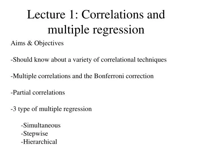
Lecture 1: Correlations and multiple regression. Aims & Objectives Should know about a variety of correlational techniques Multiple correlations and the Bonferroni correction Partial correlations 3 type of multiple regression Simultaneous Stepwise Hierarchical. Questions & techniques.

E N D
Lecture 1: Correlations and multiple regression • Aims & Objectives • Should know about a variety of correlational techniques • Multiple correlations and the Bonferroni correction • Partial correlations • 3 type of multiple regression • Simultaneous • Stepwise • Hierarchical
Questions & techniques • What is the association between a set of variables • This takes a number of multi-variate forms • Associations between a number of variables • (multiple-correlations) • Associations between 1 variable (DV) and many variables (IVs) – MODEL BUILDING • regression and partial correlations • Associations between 1 set of variables and another set of variables • canonical correlations
Correlations +1 High Vary between –1 and 1 -1 Low High Low
Types of correlation • Pearson’s (Interval and ratio data) • Spearman’s (Ordinal data) • Phi (both true dichotomies) • Tau (rating) • Biserial (Interval & dichotomised) • Point-biserial (interval & true dichotomy)
Factors affecting correlations • Outliers • Homoscedecence • Restriction of range • Multi-collinearity • Singularity
Outliers Outlier or influential point Cook’s distance of 1 or greater
Homoscedasticity When the variability of scores (errors) in one continuous variable is the same in a second variable At group level data this is Termed homogeneity of variance
Heteroscedasicity One variable is skew or the relationship is non-linear
Singularity & Multicollinearity • Singularity: • when variables are redundant, one variable is a combination of two or more other variables. • Multi-collinearity: • when variables are highly correlated (.90+). For example two measures of IQ • Problems • Logical: Don’t want to measure the same thing twice. • Statistical: Singularity prevents matrix inversion (division) as determinants = zero, for multi-collinearity determinant zero to many decimal places • Screening • Bivariate correlations • Examine SMC: large = problems • Tolerance (1 – SMC) • Solutions: • Composite score • Remove 1 variable
IQ: Multi-collinearity & Singularity Multicolinear IQ2 IQ1 Singular Memory Maths Verbal Spatial Total IQ is singular with its own sub-scales (total is a function of combining subscales One total IQ test (MD5) is multicolinear with another (MAT)
Partial correlations Partial r Neuroticism (N) = once the overlap of stress with N and the Stress with Depression is removed Semi-partial r for N = once overlap of Stress with N is removed Neuroticism Depression IV1 [N] a DV d c [Dep] b [S] IV2 Stress
Bonferroni correction • With multiple r matrix [R] or many (k) IVs in regression analysis then the possibility of chance effects increases • Correct the a level (0.05/N) • Correct for the number of effects expected by chance = a * N (0.05 * N)
Multiple regression Y B (slope) A (intercept) X
Regression assumptions • N:IVs ratio • Assume medium effect size • for Multiple Correlations N > 50 + 8m (m = N of IVs) • For simple linear regression N > 104 + m • (8/f2) + (m – 1). Where f2 = ES = .10, .15 • or f2 = .35 • f2 = R2/(1 – R2) for a more accurate estimate – Stepwise 40:1 • Outlier = Cook distance • Singularity-Multi-collinearity = SMCs • Normality = residual plots
Types of regression • Simultaneous (Standard) • No theory and enter all IV in one block • Stepwise • No theory. Allows the computer to choose on statistical ground the best sub-set of IVs to fit the equations. Capitalises on chance effects • Hierarchical (sequential)– • Theory driven. A-priori sequence of entry.
Types of regression: An example Simultaneous Age Gender Stress N Control Stepwise Age Control Hierarchical Step 1 Age Gender Step 2 Stress N Control
Venn Diagrams Age Sex Depression a b c d e Neuroticism f g Stress
Standard Regression Age Sex Depression a c e Neuroticism g Stress
Hierarchical Step 1 Age Sex Depression a b c d e Neuroticism f g Step 2 Stress
Stepwise Age Sex Depression a b c d e Neuroticism f g Stress
Stepwise Age Sex Depression a b c d e Neuroticism f g Stress
Statistical terms • B = un-standardized Beta • Beta = standardized (-1 to +1) • T-test = Is the beta significant? • R2 0-1 (amount of variance accounted for) • DR2 = Change in from one block to the next • DF = is the change in R significant? • F = Is the equation significant?