Download
1 / 36
360 likes | 543 Views
The Hyperspectral Imager for the Coastal Ocean (HICO): Sensor and Data Processing Overview. Robert Arnone, Naval Research Laboratory-Stennis Space Center Rick Gould, Naval Research Laboratory-Stennis Space Center Paul Martinolich, QinetiQ North America

E N D
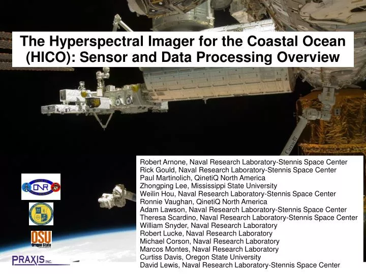
The Hyperspectral Imager for the Coastal Ocean (HICO): Sensor and Data Processing Overview Robert Arnone, Naval Research Laboratory-Stennis Space Center Rick Gould, Naval Research Laboratory-Stennis Space Center Paul Martinolich, QinetiQ North America Zhongping Lee, Mississippi State University Weilin Hou, Naval Research Laboratory-Stennis Space Center Ronnie Vaughan, QinetiQ North America Adam Lawson, Naval Research Laboratory-Stennis Space Center Theresa Scardino, Naval Research Laboratory-Stennis Space Center William Snyder, Naval Research Laboratory Robert Lucke, Naval Research Laboratory Michael Corson, Naval Research Laboratory Marcos Montes, Naval Research Laboratory Curtiss Davis, Oregon State University David Lewis, Naval Research Laboratory-Stennis Space Center
Hyperspectral Imager for the Coastal Ocean (HICO) • Sponsored as an Innovative Naval Prototype (INP) of Office of Naval Research • January 2007: HICO selected to fly on the International Space Station (ISS) • November, 2007: construction began following the Critical Design Review • August, 2008: sensor integration completed • April, 2009: shipped to Japan Aerospace Exploration Agency (JAXA) for launch • September 10, 2009: HICO launched on JAXA H-II Transfer Vehicle (HTV) • September 24, 2009: HICO installed on ISS Japanese Module Exposed Facility • HICO sensor • is first spaceborne imaging spectrometer designed to sample coastal oceans • samples coastal regions at 100 m (380 to 1000 nm: at 5.7 nm bandwidth) • has high signal-to-noise ratio to resolve the complexity of the coastal ocean Left, HICO, before integration into HREP. Right red arrow shows location of HREP on the JEM-EF. HICO is integrated and flown under the direction of DoD’s Space Test Program
HICO Goal and Objectives • Goal: build and operate the first spaceborne hyperspectral imager designed for coastal oceans • Data processing by NRL 7200 (Remote Sensing Division) and 7300 (Oceanography Division) • Other space HSI: ARTEMIS (launched this summer), Hyperion on NASA EO-1 • HICO sponsored by ONR as an Innovative Naval Prototype • Coordinated by DOD Space Test Program with NASA (Houston) • Instrument: high signal to noise, moderate spatial resolution, large area coverage • Mission planning objectives and products: • support of demonstrations of Naval utility of environmental products (ONR mission) • repeat imaging of selected coastal sites worldwide over all seasons (extended mission) • exploration of the wide range of solar illumination and viewing angles “provided” by the ISS (extended mission)
Optical Components of a Coastal Scene Multiple light paths • Scattering due to: • atmosphere • aerosols • water surface • suspended particles • bottom • Absorption due to: • atmosphere • aerosols • suspended particles • dissolved matter • Scattering and absorption are convolved Physical and biological modeling of the scene is often required to analyze the hyperspectral image. Accurate radiometric calibration of the imager is necessary to compare data to models
HICO Sensor - Stowed position spectrometer & camera Slit
Parameter Performance Rationale Spectral Range 380 to 960 nm All water-penetrating wavelengths plus Near Infrared for atmospheric correction Spectral Channel Width 5.7 nm Sufficient to resolve spectral features Number of Spectral Channels ~100 Derived from Spectral Range and Spectral Channel Width Signal-to-Noise Ratio for water-penetrating wavelengths > 200 to 1 for 5% albedo scene (10 nm spectral binning) Provides adequate Signal to Noise Ratio after atmospheric removal Polarization Sensitivity < 5% Sensor response to be insensitive to polarization of light from scene Ground Sample Distance at Nadir ~100 meters Adequate for scale of selected coastal ocean features Scene Size ~50 x 200 km Large enough to capture the scale of coastal dynamics Cross-track pointing +45 to -30 deg To increase scene access frequency Scenes per orbit 1 maximum Data volume and transmission constraints Most Requirements Derived from Aircraft Experience
HICO on Japanese Module Exposed Facility HICO Japanese Module Exposed Facility
HICO docked at ISS HICO Viewing Slit
Mission Planning with Satellite Tool Kit (STK) Combines targets, ISS attitude, ISS ephemeris, HICO FOR and constraints to produce list of all possible observations in particular time period • Constraints include: • Targets in direct sun • Angle from ISS z-axis • to Sun <= 140° • Sun specular point • exclusion angle = 30° • Sun ground elevation angle >= 25°
L0 to L1B File Generation L0 Files SOH and science data Science data Attitude data Position, velocity data Science timing data Dark subtraction 2nd order calibration Attitude, position, velocity, time SOH Data Calibrated data Geolocation L1B HDF
APS: Automated Processing System • Individual scenes are sequentially processed from the raw digital counts (Level-1) using standard parameters to a radiometrically, atmospherically, and geometrically corrected (Level-3) product within several minutes. • It further processes the data into several different temporal (daily, 8-day, monthly, and yearly) composites or averages (Level-4). • HICO repeat may preclude this normal processing • Additionally, it automatically generates quick-look ``browse'' images in JPEG format which are stored on a web. • PNG, TiFF/GeoTiFF, World File side-car file • Populates an SQL database using PostgreSQL. • It stores the Level-3 and Level-4 data in a directory-based data base in HDF format. The data base resides on a 20TB RAID array. • APS format in netCDF (v3, v4), HDF (v4, v5). HICO ΔPDR -
HICO Processing Activity in APS Level 2d: Hyperspectral Algorithm Derived Product Hyperspectral QAA At, adg, Bb, b. CHL (12) CWST - LUT Bathy, Water Optics Chl, CDOM Coastal Ocean Products Methods Level 0 Level 01a – Navigation Level 1b- Calibration Vicarious Calibration Level 1b : Calibration Multispectral Hyperspectral Level 1c – Modeled Sensor bands MODIS MERIS OCM SeaWIFS Level 2a: Sunglint Level 2b –TAFKAA Atmospheric Correction Level 2f: Cloud and Shadow Atm Correction Level 2c- : Hyperspectral L2gen- Atm Correction Atmospheric Correction Methods Level 2c: Standard APS Multispectral Algorithms Products QAA, Products At, adg, Bb, b. CHL (12) NASA: standards OC3, OC4, etc (9) Navy Products Diver Visibility Laser performance K532 Etc (6) HOPE Optimization (bathy, optics, chl, CDOM ,At, bb ..etc Level 3: Remapping Data and Creating Browse Images
HICO Data North Google Earth HICO ImageHong Kong : 10/02/09
HICO ImageBahrain: 10/02/09 HICO Data North Google Earth
Google Earth North HICO ImageYangtze River: 10/20/09 HICO Data
HICO ImageHan River: 10/21/09 HICO Data North Google Earth
HICO ImageChesapeake Bay: 10/09/09 Google Earth HICO Data
Comparison of HICO and MERIS H-CO vs MERIS at Lake Okeechobee Lt comparison Spectra Comparison • Pattern of HICO spectra overlaid on MERIS spectra • Comparison has good visual fit Lake Okeechobee
Comparison of HICO and MERIS Rrs comparison Reflectance Spectra Comparison • Cloud / Shadow Atmospheric Correction Performed • Pattern of HICO spectra overlaid on MERIS spectra • Comparison has good visual fit Lake Okeechobee
HICOSunglint Correction Module • Original ENVI Module written in IDL; modified, converted to C. • Based on the Hochberg et al. (2003) algorithm developed using 4m Ikonos imagery; Modified by Hedley et al. (2005); now modified to be automated. • NIR band used to determine amount of glint in each band (limitation: NIR should be between 700 and 910 nm) • Called as separate module from APS. • Complete hyperspectral processing. • Uses deep-water pixels only to develop regression equation • Prior to atmospheric correction • Uses NIR to derive relative spatial glint distribution • Scaled by absolute glint contribution from VIS bands
HICOSunglint Correction Module original Tested on AVIRIS HICO-proxy 20m resolution image. Input file name: aviris_20010731_r04_sc03to06.bil (short integer, BIL, 2000 lines, 512 pixels per line) • data converted to 32-bit floating point to test the deglint program. • deglint program can accept either type of data as input). display lines: 600 to 1399 (image height 800) display pixels: 0 to 511 (image width 512) Display bands: R - 57 (672.9 nm) G - 31 (523.4 nm) B - 18 (448.8 nm) NIR band: 90 (862.2 nm)
HICOSunglint Correction Module mask.jpg Classification to identify water pixels (based on NDVI computation): NDVI = (NIR – RED) / (NIR + RED) Land pixel:computed NDVI > NDVI threshold (-0.2). Water pixel:computed NDVI <= NDVI threshold (-0.2) and RED band value <= water threshold (1000). Deep-Water pixel (red):computed NDVI <= NDVI threshold (-0.2) and RED band value <= deep-water threshold (600). Shallow-Water pixel (green):computed NDVI <= NDVI threshold (-0.2) and RED band value >= deep-water threshold (600). Uses statistics from deep-water pixels for glint correction (correction applied to all bands). (the question is how to set the proper shallow-water threshold values - more tests may be needed…..)
HICOSunglint Correction Module AVIRIS HICO-proxy image (deep-water pixels) Outliers (shallow pixels?) that should not be included in regression – needs refinement Ri' = Ri - bi × (RNIR - MinNIR) Ri is visible band pixel value Ri’ is “deglinted” value
HICOSunglint Correction Module final After Glint Removal original Before Glint Removal
HICOSunglint Correction Module Before Glint Removal Wave Facet After Glint Removal
HICOSunglint Correction Module Before Glint Removal Deep Water After Glint Removal
HICOSunglint Correction Module Before Glint Removal Turbid Plume After Glint Removal
HICOSunglint Correction Module Before Glint Removal Land After Glint Removal Land values do not change
HICO ImageBahamas: 10/22/09 Radiance Bathymetry Absorption
HICO ImageKey Largo, Florida: 11/13/09 Radiance Bathymetry Absorption
Selected HICO APS Data ProductsKey Largo, Florida Kd_490 bb_551 Radiance chl_02
Near-Infrared Slope Algorithm (calculate absorption, scattering, backscattering coefficients) Assumptions • At 715-735 nm, total absorption is controlled by pure-water absorption(i.e., absorption by phytoplankton pigments, detritus, and CDOM are negligible and the spectral curve shapes are relatively flat). • The spectral shapes of b and bb are also relatively flat over this narrow wavelength range(only a 2.8% difference between b(715) and b(735), using the spectral model of Gould et al., 1999). • The C term is a constant • (C = t2 f / n2 Q = 0.047). 1 = 715 nm, 2 = 735 nm aw1,pure water absorption at 715 nm = 1.007 aw2, pure water absorption at 735 nm = 2.39 bb2 = 0.97234 bb1 t = 0.979 f/Q (665) = 0.0881 n = 1.34
Lake Okeechobee Rrs (following Cloud & Shadow atmospheric correction) some negative reflectances In clear water R: Band 62 (701.1 nm) G: Band 36 (552.2 nm) B: Band 21 (466,3 nm)
Lake Okeechobee Absorption Coefficient (m-1) Scattering Coefficient (m-1)
NRL – HICO Team NRL – DC NRL – SSC Academic • Michael Corson, PI • Robert Lucke, Lead Engineer • Bo-Cai Gao • Charles Bachmann • Ellen Bennert • Karen Patterson • Dan Korwan • Marcos Montes • Robert Fusina • Rong-Rong Li • William Snyder • Bob Arnone • Rick Gould • Paul Martinolich • Zhongping Lee • Will Hou • David Lewis • Martin Montes • Ronnie Vaughn • Theresa Scardino • Adam Lawson • Curt Davis, OSU, Project Scientist • Jasmine Nahorniak, OSU • Nick Tufillaro, OSU • Curt Vandetta, OSU • Ricardo letelier, OSU • Zhong-Ping Lee, MSU
HICO Docked on the Space Station Japanese Exposed Facility HICO Questions?