Download
1 / 23
240 likes | 415 Views
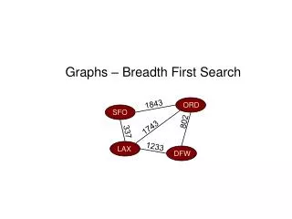
Breadth First Search. Representations of Graphs. Two standard ways to represent a graph Adjacency lists, Adjacency Matrix Applicable to directed and undirected graphs. Adjacency lists Graph G(V, E) is represented by array Adj of | V | lists

E N D
Representations of Graphs • Two standard ways to represent a graph • Adjacency lists, • Adjacency Matrix • Applicable to directed and undirected graphs. Adjacency lists • Graph G(V, E) is represented by array Adj of |V| lists • For each u V, the adjacency list Adj[u] consists of all the vertices adjacent to u in G • The amount of memory required is: (V + E)
Adjacency Matrix • A graph G(V, E) assuming the vertices are numbered 1, 2, 3, … , |V| in some arbitrary manner, then representation of G consists of: |V| × |V| matrix A = (aij) such that 1 if (i, j) E 0 otherwise • Preferred when graph is dense • |E| is close to |V|2 aij={
1 2 3 5 4 1 2 2 5 4 4 Adjacency matrix of undirected graph
Adjacency Matrix • The amount of memory required is • (V2) • For undirected graph to cut down needed memory only entries on and above diagonal are saved • In an undirected graph, (u, v) and (v, u) represents the same edge, adjacency matrix A of an undirected graph is its own transpose A = AT • It can be adapted to represent weighted graphs.
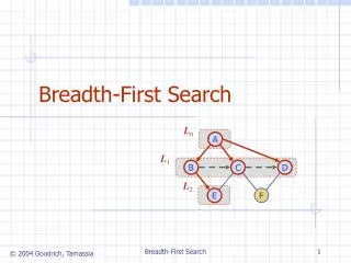
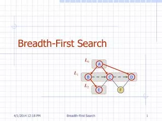
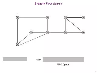
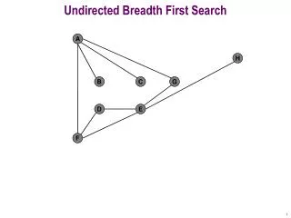
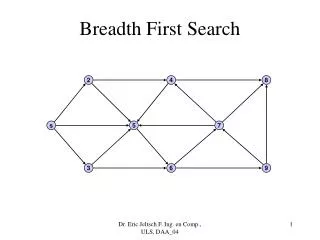
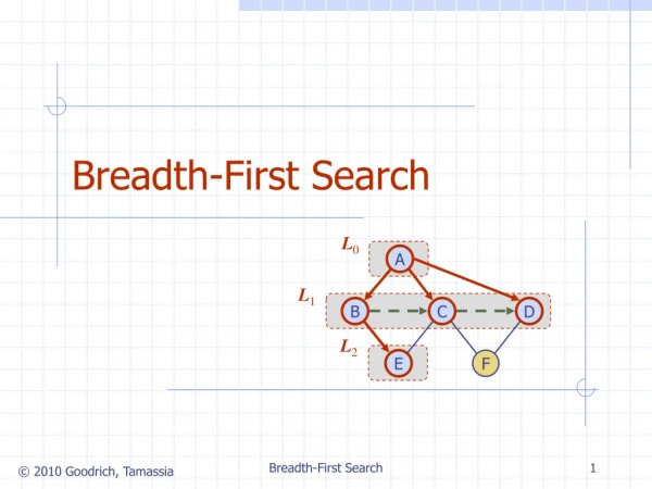
Breadth First Search • One of simplest algorithm searching graphs • A vertex is discovered first time, encountered • Let G (V, E) be a graph with source vertex s, BFS • discovers every vertex reachable from s. • gives distance from s to each reachable vertex • produces BF tree root with s to reachable vertices • To keep track of progress, it colors each vertex • vertices start white, may later gray, then black • Adjacent to black vertices have been discovered • Gray vertices may have some adjacent white vertices
Breadth First Search • It is assumed that input graph G (V, E) is represented using adjacency list. • Additional structures maintained with each vertex v V are • color[u] – stores color of each vertex • π[u] – stores predecessor of u • d[u] – stores distance from source s to vertex u
Breadth First Search BFS(G, s) 1 for each vertex u V [G] – {s} 2 do color [u] ← WHITE 3 d [u] ← ∞ 4 π[u] ← NIL 5 color[s] ← GRAY 6 d [s] ← 0 7 π[s] ← NIL 8 Q ← Ø /* Q always contains the set of GRAY vertices */ 9 ENQUEUE (Q, s) 10 while Q ≠ Ø 11 do u ← DEQUEUE (Q) 12 for each v Adj [u] 13 do if color [v] = WHITE /* For undiscovered vertex. */ 14 then color [v] ← GRAY 15 d [v] ← d [u] + 1 16 π[v] ← u 17 ENQUEUE(Q, v) 18 color [u] ← BLACK
Q Breadth First Search Except root node, s For each vertex u V(G) color [u] WHITE d[u] ∞ π [s] NIL r s t u v w x y
Q s Breadth First Search Considering s as root node color[s] GRAY d[s] 0 π [s] NIL ENQUEUE (Q, s) r s t u 0 v w x y
Q w r Breadth First Search • DEQUEUE s from Q • Adj[s] = w, r • color [w] = WHITE • color [w] ← GRAY • d [w] ← d [s] + 1 = 0 + 1 = 1 • π[w] ← s • ENQUEUE (Q, w) • color [r] = WHITE • color [r] ← GRAY • d [r] ← d [s] + 1 = 0 + 1 = 1 • π[r] ← s • ENQUEUE (Q, r) • color [s] ← BLACK r s t u 1 0 1 v w x y
Q r t x Breadth First Search • DEQUEUE w from Q • Adj[w] = s, t, x • color [s] ≠ WHITE • color [t] = WHITE • color [t] ← GRAY • d [t] ← d [w] + 1 = 1 + 1 = 2 • π[t] ← w • ENQUEUE (Q, t) • color [x] = WHITE • color [x] ← GRAY • d [x] ← d [w] + 1 = 1 + 1 = 2 • π[x] ← w • ENQUEUE (Q, x) • color [w] ← BLACK r s t u 1 0 2 1 2 v w x y
Q t x v Breadth First Search • DEQUEUE r from Q • Adj[r] = s, v • color [s] ≠ WHITE • color [v] = WHITE • color [v] ← GRAY • d [v] ← d [r] + 1 = 1 + 1 = 2 • π[v] ← r • ENQUEUE (Q, v) • color [r] ← BLACK r s t u 1 0 2 2 1 2 v w x y
r s t u 1 0 2 3 2 1 2 v w x y Q x v u Breadth First Search DEQUEUE t from Q Adj[t] = u, w, x color [u] = WHITE color [u] ← GRAY d [u] ← d [t] + 1 = 2 + 1 = 3 π[u] ← t ENQUEUE (Q, u) color [w] ≠ WHITE color [x] ≠ WHITE color [t] ← BLACK
r s t u 1 0 2 3 2 1 2 3 v w x y Q v u y Breadth First Search DEQUEUE x from Q Adj[x] = t, u, w, y color [t] ≠ WHITE color [u] ≠ WHITE color [w] ≠ WHITE color [y] = WHITE color [y] ← GRAY d [y] ← d [x] + 1 = 2 + 1 = 3 π[y] ← x ENQUEUE (Q, y) color [x] ← BLACK
r s t u 1 0 2 3 2 1 2 3 v w x y Q u y Breadth First Search DEQUEUE v from Q Adj[v] = r color [r] ≠ WHITE color [v] ← BLACK
r s t u 1 0 2 3 2 1 2 3 v w x y Q y Breadth First Search DEQUEUE u from Q Adj[u] = t, x, y color [t] ≠ WHITE color [x] ≠ WHITE color [y] ≠ WHITE color [u] ← BLACK
r s t u 1 0 2 3 2 1 2 3 v w x y Q Breadth First Search DEQUEUE y from Q Adj[y] = u, x color [u] ≠ WHITE color [x] ≠ WHITE color [y] ← BLACK
Breadth First Search • Each vertex is enqueued and dequeued atmost once • Total time devoted to queue operation is O(V) • The sum of lengths of all adjacency lists is (E) • Total time spent in scanning adjacency lists is O(E) • The overhead for initialization O(V) Total Running Time of BFS = O(V+E)
Shortest Paths • The shortest-path-distanceδ(s, v) from s to v as the minimum number of edges in any path from vertex s to vertex v. • if there is no path from s to v, then δ(s, v) = ∞ • A path of length δ(s, v) from s to v is said to be a shortest path from s to v. • Breadth First search finds the distance to each reachable vertex in the graph G (V, E) from a given source vertex s V. • The field d, for distance, of each vertex is used.
Shortest Paths • BFS-Shortest-Paths (G, s) • 1 v V • 2 d [v] ← ∞ • 3 d [s] ← 0 • 4 ENQUEUE (Q, s) • 5 whileQ ≠φ • 6 do v ← DEQUEUE(Q) • 7 for each w in Adj[v] • 8 do ifd [w] = ∞ • 9 then d [w] ← d [v] +1 • 10 ENQUEUE (Q, w)
Print Path • PRINT-PATH (G, s, v) • 1 if v= s • 2 then print s • 3 else if π[v] = NIL • 4 then print “no path froms to v exists • 5 else PRINT-PATH (G, s, π[v]) • 6 print v