Download
1 / 65
650 likes | 776 Views
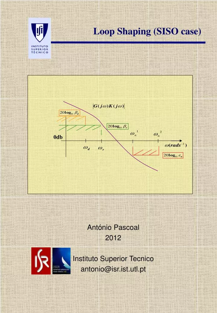
Loop Shaping (SISO case). 0db. António Pascoal 2012 Instituto Superior Tecnico antonio@isr.ist.utl.pt. r – reference signal ( to be tracked by the output y ) d – external perturbation (referred to the output) n – sensor noise e – error y – output signal u – actuation signal.

E N D
Loop Shaping (SISO case) 0db António Pascoal 2012 Instituto Superior Tecnico antonio@isr.ist.utl.pt
r – reference signal ( to be tracked by the output y) d – external perturbation (referred to the output) n – sensor noise e – error y – output signal u – actuation signal Feedback Control structure Plant Controller _
i) K(s) stabilizesG(s) Key objectives Design the controller K(s) such that ii) The output yfollows the reference signals r. iii) The system reduces the effect of external disturbance d and noise n on the output y. iv) The actuation signal u is not driven beyond limits imposed by saturation values and bandwith of the plant´s actuator. v) The system meets stability and performance requirements in the face of plant parameter uncertainty and unmodeled dynamics (robust stability and robust performance).
Control objectives Linear system superposition principle External disturbance attenuation (reducing the impact of d on y) _
S(s) – possible Bode diagram below the ‘barrier’ of –x db for 0db -x db Disturbance attenuation Y(s) D(s) S(s) – Sensitivity Function
d – sinusoidal signals Performance specs on disturbance attenuation Upper limit on Upper limit –x dband performance bandwith are problem dependent Attenuation of sinusoidal disturbances Performance bandwith Attenuation of at least –x db
d- modeled as a stationary stochastic process with spectral density y - stationary stochastic process with spectral density Energy Disturbance attenuation What happens when d is not a sinusoid?
Basic technique to reduce the energy of y: reduce Its is up to the system designer to select the level of attenuation Disturbance attenuation If spectral contents of d concentrated in the frequency band
If Disturbace attenuation Disturbance attenuation: constraints on the Loop Gain GK
Lower bound (“barrier”) on shaped by proper choice of controller K(s) Disturbance attenuation: constraints on the Loop Gain GK 0db
r- modeled as a stationary stochastic process with spectral density e - stationary stochastic process with spectral density Energia Reference following
Technique to reduce the energy of the tracking error e Reduce Its is up to the system designer to select the level of error reduction Reference following If spectral contents of d concentrated in the frequency band
Reference following Geometric constraint below the “barrier” of db for 0db db
reference following: Reference following: constraints on the Loop Gain GK If
Lower bound (“barrier”) on shaped by proper choice of controller K(s) Reference following: constraints on the Loop Gain GK 0db
n- modeled as a stationary stochastic process with spectral density y - stationary stochastic process with spectral density Energy Noise reduction
Technique to reduce the energy of y caused by the noise n: Reduce Its is up to the system designer to select the level of error reduction Noise reduction(high frequency noise) If spectral contents of n concentrated in the frequency band
upper bound (“barrier”) on shaped by proper choice of controller K(s) Noise reduction(high frequency noise) 0db
noise reduction Noise reduction: constraints on the Loop Gain GK If
Upper bound (“barrier”) on loop gain shaped by proper choice of K(s) Noise reduction: constraints on the Loop Gain GK 0db
Suppose (plant gain rolls off at high frequencies) Actuator limits _
Actuation signals too high unless the loop gain starts rolling off at frequencies below Golden rule: never try to make the closed loop bandwidth extend well above the region where there the plant gain starts to roll off below 0db. Actuator limits Suppose
Upper bound (“barrier”) on loop gain shaped by proper choice of K(s) Actuator limits Technique for limiting actuation signals Its is up to the system designer to select the parameters 0db
Putting it all together Loops Gain restrictions 0db Low frequency barriers r, d High frequency barriers n, u Goal: Shape (by appropriate choice of K(s) the LOOP GAIN G(s)K(s)so that it will meet the barrier constraints while preserving closed loop stability.
Loop Shaping – Design examples Exemple 1 . Plant (system to) be controlled G(s) . Control specifications Controller Plant _ DesignK(s) so as to stabilize G(s) and meet the following performance specifications:
i) Reduce by at least –80db the influence of d on y in the frequency band ii) Follow with error less than or equal to -40db the reference signals r in the frequency band iii) Attenuate by at least –20db the noise n in the frequency band iv) Static error in response to a unit parabola reference v) Phase Margin vi) Gain Margin Loop Shaping – Design examples Specifications
i) ii) iii Loop Shaping – Design examples Geometrical constraints; conditions i), ii), iii)
0db Loop Shaping – Design examples Loop Gain Constraints Low frequency barriers r, d High frequency barrier n
Static error in response to a unit parabola reference (possible to achieve, because G(s) has two poles at the origin) Let Loop Shaping – Design examples Condition iv)
Loop Shaping – Design examples A simple controller candidate: Checking the constraints on Loop Gain 0db Phase of The constraints are met but ….. !
Pure “PHASE LEAD” network Phaseof odb z z Loop Shaping – Design examples It is necessary to introduce some phase lead Minimum phase margin (specs): Additional phase required : real phase margin = 0 graus security factor (startbytryingsecurity factor = 0). Additional phase required: 450 Phase lead
Checking the constraints on Loop Gain Loop Shaping – Design examples New 0db Phase of Phase lead Loop Gain constraints are met and ….. NOTICE: phase lead “opens-up” the loop gain! The new loop gain barely avoids violating the noise-barrier!
Loop Shaping – Design examples Final check on stability and Gain Margin Use Nyquist’s Theorem Nyquist contour Number of open loop poles inside the Nyquist contour P=0 x x Number of encirclements around –1 N=0 -1 x Phase lead Stable! Gain Margin equals infinity!
Loop Shaping – Design examples Example 2 . Plant (simple torpedo model) G(s) . Control objectives Plant Controller _ DesignK(s) so as to stabilize G(s) and meet the following performance specifications:
ii) Attenuate by at least –40db the signals d in the frequency band iii) Follow with error smaller than or equal to -100db the signals r in the frequency band iv) Attenuate by at least –40db the noise n in the frequency band v) Phase Margin vi) Gain Margin Loop Shaping – Design examples Specifications i) Static position error = 0.
ii) iii) iv) Loop Shaping – Design examples Geometrical constraints; conditions i), ii), iii)
Condition i) Static position error (1 pure integrator in the direct path) A simple controller candidate: Loop Gain Loop Shaping – Design examples
Loop Shaping – Design examples Checking the constraints on Loop Gain +80db +40db 0db Phase of ! The constraints on the loop gain are met, but … Notice! Now it is not possible to use a phase-lead network because the open-loop plot would “open-up” and violate the noise barrier!
New Phase of Loop Shaping – Design examples The high frequency barrier does not allow for the use of a lead network – use a lag network (“gain-loss” network)! Force a new 0dB crossing point such that if the phase were not changed, the gain margin would meet the specifications (must loose -40dB at 1.0 rads-1)! use +80db +40db 0db
Phase of Loop Shaping – Design examples +80db +40db 0db NOTICE: the LAG network must introduce a loss of -40dB at 1 rads-1. But .. the zero is introduced at -10-1rads-1, not -1rads-1! WHY?So that the extra phase introduced by the lag network will not “interfere too much” around 1 rads-1.
Number of encirclements around -1 N=0 Stable! Gain Margin equals infinity! Loop Shaping – Design examples Final check on stability and Gain Margin Nyquist Theorem Nyquist Contour Number of open loop poles inside the Nyquist contour P=0 -z -p -1 x x x -1 x
Loop Shaping – Design examples Example 3 (Lunar Excursion Module – LEM)
Loop Shaping – Design examples Example 3 (Lunar Excursion Module – LEM) . Plant (vehicle controlled in attitude by gas jets and actuator; J=100 Nm/(rads-2)) Torque Input Voltage . Control objectives (attitude control) G(s) Plant Controller Attitude _ DesignK(s) so as to stabilize G(s) and meet the following performance specifications:
ii) Follow with error smaller than or equal to -40db the signals r in the frequency band iii) Attenuate by at least –40db the noise n in the frequency band v) Phase Margin iv) Gain Margin Loop Shaping – Design examples Specifications i) Static position error = 0. v) Robustness of stability with respect to a total delay in the control channel of up to 0.5 sec
ii) iii) Loop Shaping – Design examples Geometrical constraints; conditions ii), iii)
Condition i) Static position error (there are already two integrators in the direct path) A simple controller candidate: Loop Gain Loop Shaping – Design examples
Loop Shaping – Design examples Candidate Loop Gain Checking the constraints on Loop Gain (with ) 0db -40db Fase de
Loop Shaping – Design examples Checking the stability of the closed-loop system Use Nyquist’s Theorem Nyquist contour Number of open loop poles inside the Nyquist contour P=0 x x x Number of encirclements around –1 N=+2 -1 x Unstable!