Download
1 / 68
680 likes | 816 Views
O metod ě konečných prvků Lect_02.ppt. Principle of virtual work, a few simple elements. M. Okrouhlík Ústav termomechaniky, AV ČR , Praha Plzeň , 2010. Contents. Governing equations of solid continuum mechanics Fundamental ideas of finite element method (FEM)

E N D
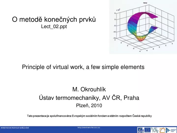
O metodě konečných prvkůLect_02.ppt Principle of virtual work, a few simple elements M. Okrouhlík Ústav termomechaniky, AV ČR, Praha Plzeň, 2010
Contents • Governing equations of solid continuum mechanics • Fundamental ideas of finite element method (FEM) • Principle of virtual displacements and work • Discretization of displacements and strains • Energy balance • Equations of equilibrium, equations of motion • Lagrangian interpolation– Lagrangian elements – generalized coordinates • Bar, beam, triangle, quadrilateral, tetrahedron and brick elements • Derivation by hand and by means of Matlab • Hermitian elements • Conditions of completeness and compatibility and convergence
Governing equations of solid continuum mechanics • Cauchy equations of motion • Kinematic relations • Constitutive relations 3 equations 6 equations 6 equations
Solution of above 15 partial differential equations • The mentioned system of partial differential equations could be analytically solved only for simple geometry and simple initial and boundary conditions. • For a long time there were attempts to solve it numerically. Historically, it was the method of finite differences which was used at first. • The solved area in space was covered by a regular mesh and the partial derivatives were replaced by a suitable difference formula at each node. • This way the partial differential equation were replaced by ordinary differential equations. • We say that the problem was discretized in space . • The resulting ordinary differential equations have (usually) to be discretized in time to find a transient solution.
Today, approximate methods of solution prevail • They are based on discretization in space and time and have numerous variants • Finite difference method • Transfer matrix method • Matrix methods • Finite element method • Displacement formulation • Force formulation • Hybrid formulation • Boundary element method • Meshless element method
Finite element method (FEM) In FEM we "fill" the structure in question by a lot of small geometrically simple parts (elements) that are connected only by their corner points (nodes).
FEM • For these elements we will derive their inertia and stiffness (damping) properties - in matrix form and will find a way how equilibrium conditions, boundary and initial conditions, and constitutive relations are satisfied. • So instead of knowing the state of stress and strain at each material point (particle) we will find a solution in nodes only.
There are many ways how the FE theory could be presented. The one, I like best, is based on the principle of virtual work.
Virtual displacements and work Stejskal, V., Okrouhlík, M.: Kmitání s Matlabem, Vydavatelství ČVUT, 2002
Práce osamělých sil Práce objemových sil Práce povrchových sil Práce vnitřních sil
Posuvy v uzlech Zatím neznámý operátor
… lagrangeovská Do hry vstupují pouze hodnoty funkce v uzlech Později se též zmíníme o hermiteovské polynomialní aproximaci – kromě hodnot funkce v uzlech uvažujeme navíc i hodnoty derivací v uzlech
Lagrangian elementsMethods of generalized coordinatesLater, we will explain another approach, namelyIsoparametric elements
(konsistentní) Say a few words about the diagonal mass matrix
For more details see: Okrouhlík, M.: Aplikovaná mechanika kontinua II, Ediční středisko ČVUT, Praha, 1989.
Summary for 1D elements • L1 … lagrangian, linear approximation function • L2 … lagrangian, quadratic • L3 … lagrangian, cubic • H3 … hermitian, cubic approximation function • H5 … hermitian, quintic See: Okrouhlík, M. – Hoeschl, C.: A contribution to the study of dispersive properties of 1D and 3D Lagrangian and Hermitian elements, Computers and structures, Vol. 49, pp. 779 – 795, 1993
How does dispersion for L1C and L1D elements depend on the mass matrix formulation The subject will be treated in more detail later. See dp_part_1.ppt
Linear displacement distribution … … constant strain element … … discontinuity at element boundaries
4-node plane elementwith bilinear displacement approximation