Download

1 / 12
120 likes | 179 Views
Incorporating the spherically symmetric potential energy. we need to deal with the radial equation that came from separation of space variables, which contains V ( r ):. the goal here is to find the function R ( r ), which tells us how the wavefunction varies with distance from the origin

E N D
Incorporating the spherically symmetric potential energy • we need to deal with the radial equation that came from separation of space variables, which contains V(r): • the goal here is to find the function R(r), which tells us how the wavefunction varies with distance from the origin • it appears that the energy of the state will depend on l but this turns out not to be the case! • a change of variables: let u(r) = rR(r) • one thing is that when calculating probabilitiesthe volume element, times the wavefunction squared, contains r2R2 := u2
Incorporating the spherically symmetric potential energy • the radial equation becomes, in terms of u(r) • this is exactly in the form of the 1d TISE • what appears here is a modified potential energy, which contains both V(r) and an additional term, dubbed the centrifugal potential • TISE has been reduced to an equivalent 1d problem, at the cost of introducing another contributionto Veff(r) • now the fun is at hand! What kind of V(r) forms to play with?
The Coulomb potential • Coulomb potential for an electron of charge e in the presence of a nucleus of charge Ze, separated by a distance • at large r, both terms die off, but centrifugal one dies quicker: < 0 • at small r, both terms blow up, but centrifugal one dominates: > 0 • there is a stable equilibrium distance, where attractive Coulomb force is ‘balanced’ by ‘repulsive’ centrifugal force • note that one could approximate the well by a harmonic potential for small disturbances from equilibrium • bound states have E < 0
Introducing a dimensionless distance, and getting long-and-short distance behavior • define an ‘inverse decay length’ • as r ∞ equation is trivial, with solution • must take B = 0 to avoid blow-up • as r 0 equation is interesting: • must take D = 0 to avoid blow-up
Peeling off those two behaviors, and defining yet another function v(r) • life seems to have gotten very very ugly, but when one puts this in • amendable to power series approach since it’s been peeled!
The power series approach to the radial equation • doing the by-now familiar process we get • rearranging, we arrive at the recurrence relation • there is no odd/even setup here, by the way
Truncating the power series • if one assumes the limiting form of the recurrence relation right from the get-go j = 0 one gets a nice approximation: • thus, there must be a jmax such that • recall what r0 was: • since jmax is an integer, so must r0/2 be one, which we call n • we have arrived at a quantization condition on the energy!
More about the principal quantum number n, etc. • therefore, l is quantized: l n = 2pn (we knew that!) • if n = l + 1 (which is its smallest possible value), the v function is a constant, and so R is a single power of r (the l –1 power) times exponential dropoff • as jmax grows, a polynomial in r with more and more powers of r enters the game, times rl−1 times exponential dropoff • normalization and probability calculations with R(r) requires the integration of r2R2(r) • we see that given an l value, n must be at least 1 bigger, and that the closer l is to n, the simpler the polynomial in r • the solutions for v(r) are the Laguerre polynomials • numbers: for electron and Z = 1 (H atom), Bohr radius is .053 nm and ground-state energy is 13.6 eV
Structure of the radial solutions I • The associated Laguerre polynomials are the v(r) functions and they are derived by differentiating the Laguerre polynomials: • since l = 0, 1, 2…, n 1, and |m| l the superscript represents the possible number of m values (the degeneracy) and the subscript can range from 0 to n 1 (the range of l values, in reverse order) • The Laguerre polynomials are given by • some Laguerre polynomials:
Structure of the radial solutions II • Some associated Laguerre polynomials: • Some normalized radial wavefunctions Rnl:
Structure of the radial solutions III • for probability calculations, use r2R2 as probability density • note that its units are m1as usual for a 1d case • some pictures of these probability densities
Building up atomic orbitals the way the chemist’s like it done • we’ll look at the 3 p orbitals: one is already up and running • this one (pz) is lobe-like along ± z, and azimuthally symmetric • it is an eigenfunction of L2 and of Lz • now consider two linear combinations: • this one is lobe-like along ± y • it is an eigenfunction of L2 but not of Lz • what operator might it be an eigenfunction of, too? • this one is lobe-like along ± x • it is an eigenfunction of L2 , and of another operator, but not of Lz