Download
1 / 28
300 likes | 534 Views
Lec 5: Capacity and LOS (Ch. 2, p.74-88). Understand capacity is the heart of transportation issues. Understand the fundamental flow of diagram Understand how a shock wave is caused

E N D
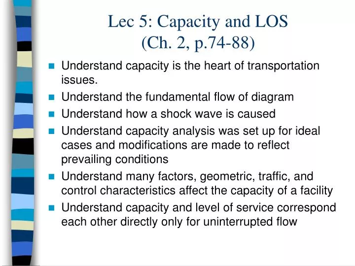
Lec 5: Capacity and LOS(Ch. 2, p.74-88) • Understand capacity is the heart of transportation issues. • Understand the fundamental flow of diagram • Understand how a shock wave is caused • Understand capacity analysis was set up for ideal cases and modifications are made to reflect prevailing conditions • Understand many factors, geometric, traffic, and control characteristics affect the capacity of a facility • Understand capacity and level of service correspond each other directly only for uninterrupted flow
Issues of traffic capacity analysis • How much traffic a given facility can accommodate? • Under what operating conditions can it accommodate that much traffic? Highway Capacity Manual (HCM) • 1950 HCM by the Bureau of Public Roads • 1965 HCM by the TRB • 1985 HCM by the TRB (Highway Capacity Software published) • 1994 updates to 1985 HCM • 1997 updates to 1994 HCM • 2000 HCM is available
Flow-density relationships Flow = (density) x (Space mean speed) Space mean speed = (flow) x (Average space headway) where Average space headway = SMS/(Average time headway) where
Fundamental diagram of traffic flow (flow vs. density) Optimal flow or capacity,qmax Mean free speed, uf Optimal speed, uo Flow (q) Speed is the slope. u = q/k Uncongested flow Congested flow Jam density, kj Optimal density, ko Density (k)
Fundamental diagram of traffic flow (SMS vs. density & SMS vs. flow) uf uf Uncongested flow SMS SMS Congested flow 0 0 kj qmax Density Flow SMS vs. density SMS vs. flow
Fundamental diagram of traffic flow and shock wave For upstream q1 Slope gives velocity uw of shock wave for q1 Flow (q) q2 Work zone For bottleneck k2 k1 kj Density (k) Queue forms upstream of the bottleneck. So we use the diagram of the upstream section
Capacity concept HCM analyses are usually for the peak (worst) 15-min period. Capacity as defined by HCM: “the maximum hourly rate at which persons or vehicles can be reasonably expectedto traverse a point or uniform segment of a lane or roadway during a given time periodunder prevailing conditions.” Sometimes using persons makes more sense, like transit Some regularity expected (capacity is not a fixed value) With different prevailing conditions, different capacity results. • Traffic • Roadway • Control
Capacity values for ideal conditions Most capacity analysis models include the determination of capacity under ideal roadway, traffic, and control conditions, that is, after having taken into account adjustments for prevailing conditions.
Factors affecting: examples Trucks occupy more space: length and gap Drivers shy away from concrete barriers
From ideal conditions to real, prevailing conditions We use adjustment factors to take into account the effect of prevailing conditions on capacity and level of service. Typically it is like… Free-flow speed: Passenger car equivalent flow rate:
Level of service “A level of service is a letter designation that describes a range of operating conditions on a particular type of facility.” LOS A (best) LOS F (worst or system breakdown)
LOS example: freeway basic sections Basic freeway segments: Segments of the freeway that are outside of the influence area of ramps or weaving areas. See Exhibit 23-3.
LOS for basic freeway segments A C B D
LOS examples near SLC LOS B LOS C or D LOS A LOS E or F
Objective of highway design Create a highway of appropriate type with dimensional values and alignment characteristics such that the resulting design service flow rate is at least as great as the traffic flow rate during the peak 15-min period of the design hour, but not greater enough as to represent extravagance or waste Why the peak 15-min period? Traffic flow fluctuates, but it is known from previous studies that it is stable for about 15 minutes.
Service flow rates vs. service volumes What is used for analysis is service flow rate. The actual number of vehicles that can be served during one peak hour is service volume. This reflects the peaking characteristic of traffic flow. Stable flow SFE Unstable flow E F Flow D C SFA SVi = SFi * PHF B A Density
Acceptable degree of congestion Balance need (demand) and resources available (supply) to determine the degree of congestion for design.